|
Size: 13727
Comment:
|
← Revision 48 as of 2017-01-10 19:37:47 ⇥
Size: 15220
Comment:
|
| Deletions are marked like this. | Additions are marked like this. |
| Line 9: | Line 9: |
| PLS is a free toolbox that is available at Baycrest (https://www.rotman-baycrest.on.ca/index.php?section=84). The PLS code is written entirely in MATLAB (Mathworks Inc) and can be downloaded from https://www.rotman-baycrest.on.ca/index.php?section=345. To cite PLS Toolbox, please see the “References” section of this tutorial. | PLS is a free toolbox that is a part of [[https://www.rotman-baycrest.on.ca/index.php?section=84|Baycrest, University of Toronto]]. The PLS code is written entirely in MATLAB (Mathworks Inc) and can be downloaded from https://www.rotman-baycrest.on.ca/index.php?section=345. To cite PLS Toolbox, please see the “References” section of this tutorial. |
| Line 12: | Line 12: |
| Partial Least Squares (PLS) analysis is a multivariate statistical technique that is used to find the relationship between two blocks of variables. PLS that has various applications and types (Krishnan et al., 2011); however, the focus of this tutorial is on Mean-Centered PLS analysis, which is a common type of PLS while working with neuroimaging data. In this type of PLS analysis, one data block is neural activity (e.g. MEG measurements/source data here) while the other one is the experiment design (e.g. different groups/conditions). | Partial Least Squares (PLS) analysis is a multivariate statistical technique that is used to find the relationship between two blocks of variables. PLS has various applications and types (Krishnan et al., 2011); however, the focus of this tutorial is on Mean-Centered PLS analysis, which is a common type of PLS while working with neuroimaging data. In this type of PLS analysis, one data block is neural activity (e.g. MEG measurements/source data here) while the other one is the experiment design (e.g. different groups/conditions). |
| Line 16: | Line 16: |
| For this purpose, we take the neural activity as one data block, matrix X, where the rows of matrix X are observations (participants/trials) nested in conditions or groups, and the columns of X are variables that are arranged in a way that time scales are nested within sources. The other data block, matrix Y, is a matrix of dummy coding that is related to experimental design (different groups or conditions) (Krishnan et al., 2011). | For this purpose, we take the neural activity as one data block, matrix X, where the rows of matrix X are observations (participants/trials) nested in conditions or groups, and the columns of X are variables (time scales nested within sources). The other data block, matrix Y, is a matrix of dummy coding that corresponds to experimental design (different groups or conditions) (Krishnan et al., 2011). |
| Line 18: | Line 18: |
| PLS analysis first calculates a mean-centered matrix using matrices X and Y. Then, singular value decomposition (SVD) is applied on the mean-centered matrix. The outcome of PLS analysis is a set of latent variables that are in fact linear combinations of initial variables of the two data blocks that maximally covary with the resulting contrasts (Krishnan et al., 2011, Misic et al., 2016). | PLS analysis first calculates a mean-centered matrix using matrices X and Y. Then, singular value decomposition (SVD) is applied on the mean-centered matrix. The outcome of PLS analysis is a set of latent variables that are in fact linear combinations of initial variables of the two data blocks that maximally covary with the corresponding contrasts (Krishnan et al., 2011, Mišić et al., 2016). More specifically, each latent variable consists of a set of singular values that describe the effect size, as well as a set of singular vectors, or ''weights'', that define the contribution of each initial variable to the latent variables (Mišić et al., 2016). |
| Line 20: | Line 20: |
| Finally, the statistical significance of a latent variable is defined by a p-value calculated from permutation test. In addition, bootstrapping is used to assess the reliability of each original variable (e.g. a source at a time point) that contributes to the latent variable. Bootstrap ratios are calculated for each original variable for this purpose. More specifically, each latent variable consists of a set of singular values that describe the effect size, as well as a set of singular vectors, ''or weights'', that define the contribution of each initial variable to the latent variables. The ratio of these weights to the standard errors estimated from bootstrapping is called bootstrap ratio. Therefore, the larger the magnitude of a bootstrap ratio, the larger the weight (i.e. contribution to the latent variable) and the smaller the standard error (i.e. higher stability) (McIntosh and Lobaugh, 2004, Misic et al., 2016). Bootstrap ratio can be equivalent to a z-score if we have an approximately normal bootstrap distribution (Efron and Tibshirani, 1986). | Finally, the statistical significance of a latent variable is defined by a p-value calculated from permutation test. In addition, bootstrapping is used to assess the reliability of each original variable (e.g. a source at a time point) that contributes to the latent variable. Bootstrap ratios are calculated for each original variable for this purpose. Bootstrap ratio is the ratio of the weights to the standard errors estimated from bootstrapping. Therefore, the larger the magnitude of a bootstrap ratio, the larger the weight (i.e. contribution to the latent variable) and the smaller the standard error (i.e. higher stability) (McIntosh and Lobaugh, 2004, Mišić et al., 2016). Bootstrap ratio can be equivalent to a z-score if we have an approximately normal bootstrap distribution (Efron and Tibshirani, 1986). |
| Line 33: | Line 33: |
| * After you found all the averages across subjects, continue with [[http://neuroimage.usc.edu/brainstorm/Tutorials/VisualGroup#Subject_averages:_Filter_and_normalize|Section 7]] and filter the signals below 32Hz and extract time as it is explained. However, [[http://neuroimage.usc.edu/brainstorm/Tutorials/VisualGroup#Sources-2|when filtering the sources]], __do not__ normalize the __source__ values with respect to baseline (i.e. __do not__ find z-score). | * After you found all the averages across subjects, continue with [[http://neuroimage.usc.edu/brainstorm/Tutorials/VisualGroup#Subject_averages:_Filter_and_normalize|Section 7]] and filter the signals below 32Hz and extract time as it is explained. However, [[http://neuroimage.usc.edu/brainstorm/Tutorials/VisualGroup#Sources-2|when filtering the sources]], __do not__ normalize the __source__ values with respect to the baseline (i.e. __do not__ find z-score). |
| Line 38: | Line 38: |
| There are two PLS processes available in Brainstorm: * You can run PLS analysis for __only two conditions__ through the Process2 tab at the bottom of the Brainstorm window. | There are two PLS processes available in Brainstorm: |
| Line 40: | Line 40: |
| * You can run PLS analysis for __only two conditions__ through the Process2 tab at the bottom of the Brainstorm window. | |
| Line 44: | Line 45: |
| * '''Input: '''the input files are the source data from different conditions. Number of samples per condition must be the same for all conditions. In order to find meaningful results from PLS statistical analysis, each of the conditions should at least contain 5 observations/trials. | * '''Input: '''the input files are the source data from different conditions. Number of observations/trials per condition must be the same for all conditions. Make sure you have enough observations/trials per condition in order to get meaningful results from statistical tests. |
| Line 66: | Line 67: |
| Run the process when the options are set. The process will take some time depending on the number of files, number of permutations and bootstraps. The results are then saved in '''Group Analysis > Intra-Subject''' folder. | Run the process when the options are set. The process will take some time depending on the number of files, number of permutations and number of bootstraps. The results are then saved in '''Group Analysis > Intra-Subject''' folder. |
| Line 73: | Line 74: |
| * '''PLS : Contrast: '''You can first look at the contrast between two conditions: Double-click on the contrast file. The contrast is shown in the form of time series; however, the x-axis is not actual time. In fact, the integer numbers show the number of conditions (e.g. 1 for condition 1 or “Faces” and 2 for Condition 2 or “Scrambled Faces”) and the non-integer ones should be ignored.<<BR>><<BR>> {{attachment:contrast.gif}} | * '''PLS : Contrast: '''You can first look at the contrast between two conditions: Double-click on the contrast file. The contrast is shown in the form of time series; however, the x-axis is not actual time. In fact, the integer numbers on time axis show the number of conditions (e.g. 1 for condition 1 or “Faces” and 2 for Condition 2 or “Scrambled Faces”) and the non-integer ones should be ignored.<<BR>><<BR>> {{attachment:contrast.gif}} |
| Line 82: | Line 83: |
| * '''PLS: Bootstrap ratio: '''This file is saved in the format of source maps. Double-click on open the file. The colormap shows bootstrap ratios for each source at each time point. There are some important points you should keep in mind when working with bootstrap ratios: | * '''PLS: Bootstrap ratio: '''This file is saved in the format of source maps. Double-click on the file and open it. The colormap shows bootstrap ratios for each source at each time point. There are some important points you should keep in mind when working with bootstrap ratios: |
| Line 117: | Line 118: |
| * Enter the number of conditions and the number of subjects (files) per condition. | * Define the number of conditions and the number of subjects/trials per condition. |
| Line 119: | Line 120: |
| * The process will take some time. The results are displayed in the same way as before; however, you may have more bootstrap ratio files for different latent variables depending on the number of conditions you have. In this example, we have 2 latent variables.<<BR>><<BR>> {{attachment:results_overview2.gif}} |
* The process will take some time. The results are displayed in the same way as before; however, you may have more bootstrap ratio files for different latent variables depending on the number of conditions you have. In this example, we have 2 latent variables.<<BR>><<BR>> {{attachment:results_overview2.gif}} |
| Line 125: | Line 124: |
| * Check the p-values first to detect the significant latent variables. Each latent variable will have a p-value that indicates whether the related effect (or contrast) is significant or not. In this example, only latent variable 1 (LV1) is significant.<<BR>><<BR>> {{attachment:p_value2.gif}} |
* Check the p-values first to detect the significant latent variables. Each latent variable will have a p-value that indicates whether the related effect (or contrast) is significant or not. In this example, only latent variable 1 (LV1) is significant.<<BR>><<BR>> {{attachment:p_value2.gif}} |
| Line 131: | Line 128: |
| * Open the contrast file and focus on the contrasts (effects) related to the significant latent variables. | * Open the contrast file and focus on the contrasts (effects) related to the significant latent variables. LV1 (green) is the significant latent variable in this example, which discriminates condition 2 (scrambled faces) from the other conditions (famous faces and unfamiliar faces).<<BR>><<BR>> {{attachment:contrast2.gif}} <<BR>> * Keep the bootstrap ratio files for significant latent variables and delete the rest. Bootstrap ratios should be interpreted in the same way as it was explained above. Bootstrap ratio of a latent variable (e.g. LV(x) ) shows the pattern of brain activity that corresponds to the contrast defined by the same latent variable ( LV(x) ). == References == 1. Efron B, Tibshirani R (1986). "Bootstrap methods for standard errors, confidence intervals and other measures of statistical accuracy." ''Stat. Sci. 1'', 54– 77. 1. Krishnan A, Williams LJ, McIntosh AR, Abdi H (2011). "Partial Least Squares (PLS) methods for neuroimaging: a tutorial and review." ''Neuroimage, 56(2)'', 455-475. 1. McIntosh AR, Bookstein F, Haxby J, Grady C (1996). "Spatial pattern analysis of functional brain images using partial least squares." ''Neuroimage 3'', 143–157. 1. McIntosh AR, Lobaugh NJ (2004). "Partial least squares analysis of neuroimaging data: applications and advances." ''Neuroimage 23'', S250–S263. 1. Mišić B, Dunkley BT, Sedge PA, Da Costa L, Fatima Z, Berman MG, ... & Pang EW (2016). "Post-traumatic stress constrains the dynamic repertoire of neural activity." ''The Journal of Neuroscience, 36(2)'', 419-431. ---- |
Partial Least Squares (PLS)
Authors: Golia Shafiei
This tutorial explains the concept of Partial Least Squares (PLS) analysis in general, which was first introduced to the neuroimaging community in 1996 (McIntosh et al., 1996). In addition, we illustrate how to use PLS process on a sample data in Brainstorm.
Contents
License
PLS is a free toolbox that is a part of Baycrest, University of Toronto. The PLS code is written entirely in MATLAB (Mathworks Inc) and can be downloaded from https://www.rotman-baycrest.on.ca/index.php?section=345. To cite PLS Toolbox, please see the “References” section of this tutorial.
Introduction
Partial Least Squares (PLS) analysis is a multivariate statistical technique that is used to find the relationship between two blocks of variables. PLS has various applications and types (Krishnan et al., 2011); however, the focus of this tutorial is on Mean-Centered PLS analysis, which is a common type of PLS while working with neuroimaging data. In this type of PLS analysis, one data block is neural activity (e.g. MEG measurements/source data here) while the other one is the experiment design (e.g. different groups/conditions).
PLS analysis is based on extracting the common information between the two data blocks by finding a correlation matrix and linear combinations of variables in both data blocks that have maximum covariance with one another. In the example provided here, we find a contrast between different conditions as well as patterns of brain activity that maximally covary with that specific contrast.
For this purpose, we take the neural activity as one data block, matrix X, where the rows of matrix X are observations (participants/trials) nested in conditions or groups, and the columns of X are variables (time scales nested within sources). The other data block, matrix Y, is a matrix of dummy coding that corresponds to experimental design (different groups or conditions) (Krishnan et al., 2011).
PLS analysis first calculates a mean-centered matrix using matrices X and Y. Then, singular value decomposition (SVD) is applied on the mean-centered matrix. The outcome of PLS analysis is a set of latent variables that are in fact linear combinations of initial variables of the two data blocks that maximally covary with the corresponding contrasts (Krishnan et al., 2011, Mišić et al., 2016). More specifically, each latent variable consists of a set of singular values that describe the effect size, as well as a set of singular vectors, or weights, that define the contribution of each initial variable to the latent variables (Mišić et al., 2016).
Finally, the statistical significance of a latent variable is defined by a p-value calculated from permutation test. In addition, bootstrapping is used to assess the reliability of each original variable (e.g. a source at a time point) that contributes to the latent variable. Bootstrap ratios are calculated for each original variable for this purpose. Bootstrap ratio is the ratio of the weights to the standard errors estimated from bootstrapping. Therefore, the larger the magnitude of a bootstrap ratio, the larger the weight (i.e. contribution to the latent variable) and the smaller the standard error (i.e. higher stability) (McIntosh and Lobaugh, 2004, Mišić et al., 2016). Bootstrap ratio can be equivalent to a z-score if we have an approximately normal bootstrap distribution (Efron and Tibshirani, 1986).
PLS analysis was explained in general in this section. However, this tutorial assumes that the users are already familiar with basics of PLS analysis. If PLS is new to you or if you want to read more about PLS and its applications in details, please refer to the articles introduced in “References” section.
Download and installation
In order to run PLS process in Brainstorm, the PLS Toolbox must be downloaded from here and added to MATLAB pathway.
Data, Pre-Processing and Source Analysis
The data processed here is the same dataset that is used in MEG visual tutorial: Single subject and MEG visual tutorial: Group analysis. This dataset consists in simultaneous MEG/EEG recordings of 19 subjects performing a simple visual task on a large number of famous, unfamiliar and scrambled faces. The detailed presentation of experiment is available in the MEG visual tutorial: Single Subject.
You can follow this tutorial after processing the data as illustrated in MEG visual tutorial: Single Subject. Then:
Find the subject averages as it is explained in MEG visual tutorial: Group analysis by following the steps in the visual group analysis up to Section 7: Subject averages: Filter and normalize.
After you found all the averages across subjects, continue with Section 7 and filter the signals below 32Hz and extract time as it is explained. However, when filtering the sources, do not normalize the source values with respect to the baseline (i.e. do not find z-score).
At this point, continue with the rest of the group analysis tutorial: Project sources on template and apply spatial smoothing on the source maps.
- Data is now ready for PLS analysis.
Running PLS
There are two PLS processes available in Brainstorm:
You can run PLS analysis for only two conditions through the Process2 tab at the bottom of the Brainstorm window.
You can also run PLS analysis for more than two conditions through the Process1 tab at the bottom of the Brainstorm window. This option is explained in the “Advanced” section of this tutorial.
Both of these two processes work in a similar way:
Input: the input files are the source data from different conditions. Number of observations/trials per condition must be the same for all conditions. Make sure you have enough observations/trials per condition in order to get meaningful results from statistical tests.
Note: You can also run PLS analysis on sensor level data (channel data). However, the results will not be as meaningful and useful as the ones from source level data.
Output: the output files include bootstrap ratios and p-values for all latent variables. In addition, you can look at the contrast between conditions (groups and/or experimental tasks) for each latent variable. The output files are explained in details in the following sections.
We will continue with explaining the PLS process for only two conditions from now and we will leave PLS process for more conditions for the Advanced section of this tutorial.
Select files
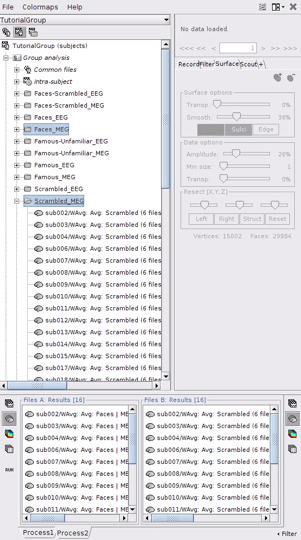
- Select the process2 tab at the bottom of Brainstorm window.
Drag and drop 16 source files from Group_analysis/Faces-MEG to the left (Files A).
Drag and drop 16 source files from Group_analysis/Scrambled-MEG to the right (Files B).
Note that the number of files in each window (“A” and “B”) must be the same.
Run PLS
- In Process2, click on [Run].
Select process Test > Partial Lest Squares (PLS). This opens the Pipeline editor window with the PLS process for two conditions.
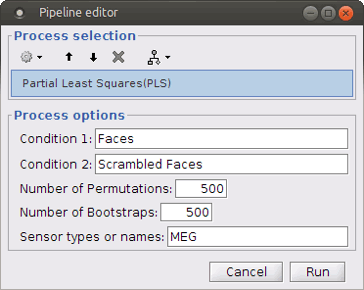
“Condition 1” and “Condition 2”: Name of the two input conditions: “Condition 1” and “Condition 2” are related to files in windows “A” and “B” of “Process2” tab, respectively. We can use “Faces” and “Scrambled Faces” as the condition names here.
Number of Permutations: Indicates the number of permutations you want to run in PLS.
Number of Bootstraps: Indicates the number of bootstraps you want to run in PLS.
Sensor types or name: Indicates the type of sensors that has been used for source localization (e.g. MEG or EEG). This will occur in the result file name as well.
Run the process when the options are set. The process will take some time depending on the number of files, number of permutations and number of bootstraps. The results are then saved in Group Analysis > Intra-Subject folder.
PLS Results
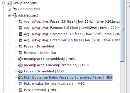
Output files include contrast between conditions, p-value of the latent variable and bootstrap ratios:
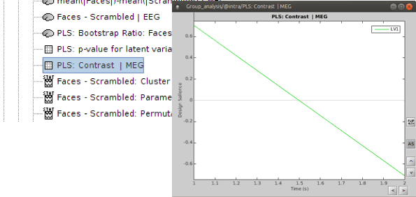
PLS : Contrast: You can first look at the contrast between two conditions: Double-click on the contrast file. The contrast is shown in the form of time series; however, the x-axis is not actual time. In fact, the integer numbers on time axis show the number of conditions (e.g. 1 for condition 1 or “Faces” and 2 for Condition 2 or “Scrambled Faces”) and the non-integer ones should be ignored.
PLS: p-value for latent variable: if you double click on this files, you will see a table containing the p-value of the latent variable that is related to the contrast shown above. A significant latent variable means the contrast observed between two conditions is also significant.
Note: You will see two numbers in the table for p-value of the latent variable when you run PLS for two conditions. Ignore the second one.

PLS: Bootstrap ratio: This file is saved in the format of source maps. Double-click on the file and open it. The colormap shows bootstrap ratios for each source at each time point. There are some important points you should keep in mind when working with bootstrap ratios:
Bootstrap ratios show how reliably each source is contributing to the observed contrast and latent variable at each time point. A bootstrap ratio larger than 2.58 is considered reliable. Therefore, adjust the amplitude of bootstrap ratios to 25%-26% to be able to see the reliable signals. For this, choose “Surface” tab from Brainstorm window and adjust the “Amplitude”.
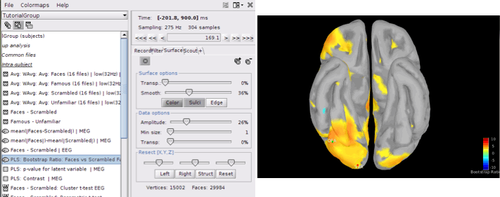
- Do not display absolute values of the signals. Make sure “Absolute Values” is not selected in the colormap menu for this figure. The sign of bootstrap ratio is important since positive bootstrap ratios express the contrast as is, while bootstrap ratios with negative values express the opposite contrast.
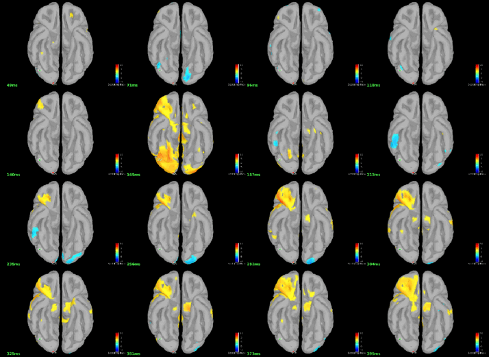
You can display the results at different time points using contact sheet.
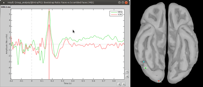
You can also define regions of interest as usual: OFA (Occipital Face Area), V1.
Advanced Option
You can run PLS for more than 2 conditions through Process1 tab. However, you should be careful when arranging the files in this option. We will use the same dataset to illustrate how to use this option in Brainstorm.
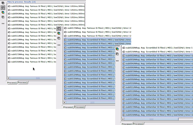
- Select the Process1 tab at the bottom of Brainstorm window.
Drag and drop 16 source maps from Group_analysis/Famous-MEG to the Process1 window.
Drag and drop 16 source maps from Group_analysis/Scrambled-MEG to the Process1 window under the previous source maps.
Finally, drag and drop 16 source maps from Group_analysis/Unfamiliar-MEG at the end of previous files.
- Make sure you have the same number of files for each condition.
Note: PLS processes the data in “subject in condition” format. Therefore, all files from the same condition must be placed in the process window at once and files from the second condition must be added to the end of first condition, and so on for the rest of the conditions.
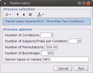
Run process Test > Partial Least Squares (PLS) – More than Two Condition.
- Define the number of conditions and the number of subjects/trials per condition.
The other options are the same as explained above.
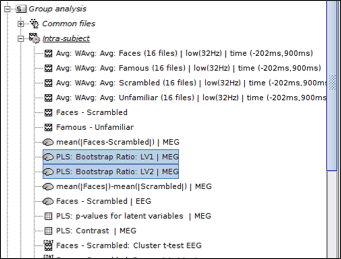
The process will take some time. The results are displayed in the same way as before; however, you may have more bootstrap ratio files for different latent variables depending on the number of conditions you have. In this example, we have 2 latent variables.
Check the p-values first to detect the significant latent variables. Each latent variable will have a p-value that indicates whether the related effect (or contrast) is significant or not. In this example, only latent variable 1 (LV1) is significant.

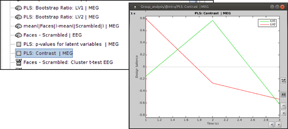
Open the contrast file and focus on the contrasts (effects) related to the significant latent variables. LV1 (green) is the significant latent variable in this example, which discriminates condition 2 (scrambled faces) from the other conditions (famous faces and unfamiliar faces).
- Keep the bootstrap ratio files for significant latent variables and delete the rest. Bootstrap ratios should be interpreted in the same way as it was explained above. Bootstrap ratio of a latent variable (e.g. LV(x) ) shows the pattern of brain activity that corresponds to the contrast defined by the same latent variable ( LV(x) ).
References
Efron B, Tibshirani R (1986). "Bootstrap methods for standard errors, confidence intervals and other measures of statistical accuracy." Stat. Sci. 1, 54– 77.
Krishnan A, Williams LJ, McIntosh AR, Abdi H (2011). "Partial Least Squares (PLS) methods for neuroimaging: a tutorial and review." Neuroimage, 56(2), 455-475.
McIntosh AR, Bookstein F, Haxby J, Grady C (1996). "Spatial pattern analysis of functional brain images using partial least squares." Neuroimage 3, 143–157.
McIntosh AR, Lobaugh NJ (2004). "Partial least squares analysis of neuroimaging data: applications and advances." Neuroimage 23, S250–S263.
Mišić B, Dunkley BT, Sedge PA, Da Costa L, Fatima Z, Berman MG, ... & Pang EW (2016). "Post-traumatic stress constrains the dynamic repertoire of neural activity." The Journal of Neuroscience, 36(2), 419-431.
