Partial Least Squares (PLS)
Authors: Golia Shafiei
This tutorial explains the concept of Partial Least Squares (PLS) analysis in general, which was first introduced to the neuroimaging community in 1996 (McIntosh et al., 1996). In addition, we illustrate how to use PLS process on a sample data in Brainstorm.
Contents
License
PLS is a free toolbox that is available at Baycrest (https://www.rotman-baycrest.on.ca/index.php?section=84). The PLS code is written entirely in MATLAB (Mathworks Inc) and can be downloaded from https://www.rotman-baycrest.on.ca/index.php?section=345. To cite PLS Toolbox, please see the “References” section of this tutorial.
Introduction
Partial Least Squares (PLS) analysis is a multivariate statistical technique that is used to find the relationship between two blocks of variables. PLS that has various applications and types (Krishnan et al., 2011); however, the focus of this tutorial is on Mean-Centered PLS analysis, which is a common type of PLS while working with neuroimaging data. In this type of PLS analysis, one data block is neural activity (e.g. MEG measurements/source data here) while the other one is the experiment design (e.g. different groups/conditions).
PLS analysis is based on extracting the common information between the two data blocks by finding a correlation matrix and linear combinations of variables in both data blocks that have maximum covariance with one another. In the example provided here, we find a contrast between different conditions as well as patterns of brain activity that maximally covary with that specific contrast.
For this purpose, we take the neural activity as one data block, matrix X, where the rows of matrix X are observations (participants/trials) nested in conditions or groups, and the columns of X are variables that are arranged in a way that time scales are nested within sources. The other data block, matrix Y, is a matrix of dummy coding that is related to experimental design (different groups or conditions) (Krishnan et al., 2011).
PLS analysis first calculates a mean-centered matrix using matrices X and Y. Then, singular value decomposition (SVD) is applied on the mean-centered matrix. The outcome of PLS analysis is a set of latent variables that are in fact linear combinations of initial variables of the two data blocks that maximally covary with the resulting contrasts (Krishnan et al., 2011, Misic et al., 2016).
Finally, the statistical significance of a latent variable is defined by a p-value calculated from permutation test. In addition, bootstrapping is used to assess the reliability of each original variable (e.g. a source at a time point) that contributes to the latent variable. Bootstrap ratios are calculated for each original variable for this purpose. More specifically, each latent variable consists of a set of singular values that describe the effect size, as well as a set of singular vectors, or weights, that define the contribution of each initial variable to the latent variables. The ratio of these weights to the standard errors estimated from bootstrapping is called bootstrap ratio. Therefore, the larger the magnitude of a bootstrap ratio, the larger the weight (i.e. contribution to the latent variable) and the smaller the standard error (i.e. higher stability) (McIntosh and Lobaugh, 2004, Misic et al., 2016). Bootstrap ratio can be equivalent to a z-score if we have an approximately normal bootstrap distribution (Efron and Tibshirani, 1986).
PLS analysis was explained in general in this section. However, this tutorial assumes that the users are already familiar with basics of PLS analysis. If PLS is new to you or if you want to read more about PLS and its applications in details, please refer to the articles introduced in “References” section.
Download and installation
In order to run PLS process in Brainstorm, the PLS Toolbox must be downloaded from here and added to MATLAB pathway.
Data, Pre-Processing and Source Analysis
The data processed here is the same dataset that is used in MEG visual tutorial: Single subject and MEG visual tutorial: Group analysis. This dataset consists in simultaneous MEG/EEG recordings of 19 subjects performing a simple visual task on a large number of famous, unfamiliar and scrambled faces. The detailed presentation of experiment is available in the MEG visual tutorial: Single Subject.
You can follow this tutorial after processing the data as illustrated in MEG visual tutorial: Single Subject. Then:
Find the subject averages as it is explained in MEG visual tutorial: Group analysis by following the steps in the visual group analysis up to Section 7: Subject averages: Filter and normalize.
After you found all the averages across subjects, continue with Section 7 and filter the signals below 32Hz and extract time as it is explained. However, when filtering the sources, do not normalize the source values with respect to baseline (i.e. do not find z-score).
At this point, continue with the rest of the group analysis tutorial: Project sources on template and apply spatial smoothing on the source maps.
- Data is now ready for PLS analysis.
Running PLS
There are two PLS processes available in Brainstorm: * You can run PLS analysis for only two conditions through the Process2 tab at the bottom of the Brainstorm window.
You can also run PLS analysis for more than two conditions through the Process1 tab at the bottom of the Brainstorm window. This option is explained in the “Advanced” section of this tutorial.
Both of these two processes work in a similar way:
Input: the input files are the source data from different conditions. Number of samples per condition must be the same for all conditions. In order to find meaningful results from PLS statistical analysis, each of the conditions should at least contain 5 observations/trials.
Note: You can also run PLS analysis on sensor level data (channel data). However, the results will not be as meaningful and useful as the ones from source level data.
Output: the output files include bootstrap ratios and p-values for all latent variables. In addition, you can look at the contrast between conditions (groups and/or experimental tasks) for each latent variable. The output files are explained in details in the following sections.
We will continue with explaining the PLS process for only two conditions from now and we will leave PLS process for more conditions for the Advanced section of this tutorial.
Select files
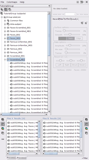
- Select the process2 tab at the bottom of Brainstorm window.
Drag and drop 16 source files from Group_analysis/Faces-MEG to the left (Files A).
Drag and drop 16 source files from Group_analysis/Scrambled-MEG to the right (Files B).
Note that the number of files in each window (“A” and “B”) must be the same.

Run PLS
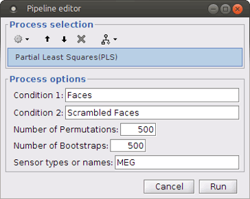
- In Process2, click on [Run].
Select process Test > Partial Lest Squares (PLS). This opens the Pipeline editor window with the PLS process for two conditions.
