|
Size: 15561
Comment:
|
Size: 15587
Comment:
|
| Deletions are marked like this. | Additions are marked like this. |
| Line 116: | Line 116: |
| * Add the process "'''Test > Difference of means'''", select the option "'''Arithmetic average'''". <<BR>>The option "weighted average" has no importance because we are averaging only single trials.<<BR>><<BR>> {{attachment:diff_mean_process.gif}} | * Add the process "'''Test > Difference of means'''", select the option "'''Arithmetic average'''". <<BR>>The option "weighted average" has no importance because we are averaging only single trials.<<BR>><<BR>> {{attachment:diff_mean_process.gif||height="358",width="310"}} |
Tutorial 25: Difference
Authors: Francois Tadel, Elizabeth Bock, Dimitrios Pantazis, Richard Leahy, Sylvain Baillet
In this auditory oddball experiment, we would like to explore what are the significant differences between the brain response to the deviant or standard beeps, time sample by time sample. To do this we will be essentially contrasting the values we obtained for both conditions, and testing if the results are significantly different from zero.
This tutorial focuses only on the first part of this problem: the contrast. Computing a difference between two condition A and B sounds trivial, but it requires some reflection when it comes to interpreting the sign of the subtraction of two signals oscillating around zero. Several options are available, we will try to explain to which application cases they correspond. The statistical significance will be discussed in the next tutorial.
Contents
Sign of the signals
First we need to define on which signals we want to compute the difference: sensor recordings, constrained sources (one signal per grid point) or unconstrained sources (three signals per grid point). For the first two we can compare the signals oscillating around zero or their absolute value, for unconstrained sources we have the additional option to use the norm of the three orientations.
Using the rectified signals (absolute value) gives us an idea of the amount of activity in one particular brain region, but alters the frequency information and therefore cannot be used for time-frequency or connectivity analysis. Additionally, the rectified signals are not always appropriate to detect effects between different experimental conditions, as illustrated in the next section.
In general, you should not apply an absolute value (or a norm) explicitly to your data. The only application cases for rectified signals are the display of the cortical maps, the comparison of magnitudes between conditions and the group analysis, and in all three cases the absolute value can be applied on the fly.
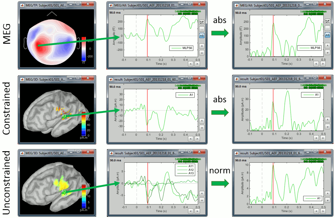
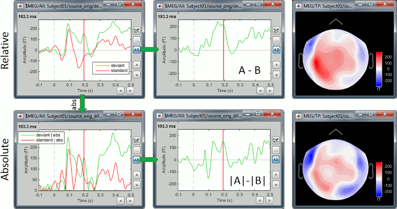
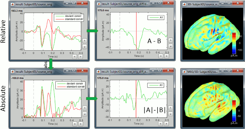
Now let's consider the two conditions for each available option. The examples below show the difference (deviant-standard) for one signal only, corresponding to the auditory cortex. The operator |x| represents the absolute value of x (i.e. the magnitude of x).
MEG/EEG sensor
We always observe important differences between (A-B) and (|A|-|B|). In the absolute case the amplitude of the difference is not representative of the distance between the green curve (deviant) and the red curve (standard). In general, the sign of the signal recorded by any MEG or EEG sensor is meaningful and we need to keep it in the analysis to account for the differences between conditions.
Never use an absolute value on sensor data.
Constrained sources
We also observe important differences between (A-B) and (|A|-|B|). At 175ms, we reach the highest distance between the red and green curves, but it corresponds to a zero in the rectified difference.
(A-B): Correct amplitude, ambiguous sign.
This measure represents better the distance between the two conditions curves. However, its sign is ambiguous and cannot be used to claim that "the brain response is stronger in condition A than in condition B" (|A|>|B|, cases a/b/e in the table below) or "is stronger in condition B than in condition A" (|B|>|A|, cases c/d). As illustrated in the source estimation tutorial, the sign of the current density maps depends on the orientation of the source.
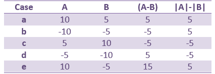
This is an appropriate measure to use when the polarity of the signal is important to you, for example when suppression of a negative peak (A-B<0) would be viewed differently than suppression of a positive peak (A-B>0) or a polarity change (sign(A) different from sign(B)).
- Suppression of positive signals from A to B (case a) produces the same value as an increase in the negative signal from A to B (case d). Similarly cases b and c will produce the same value. For this reason interpretation of the results requires that you also examine the actual polarities of the two signals at locations in time and space where significant effects are detected.
|A|-|B|: Ambiguous amplitude, meaningful sign.
- This measure is insensitive to polarity so not adapted to represent the distance between the two conditions, but its sign is meaningful.
- The sign indicates the direction of magnitude change and avoids the ambiguity encountered in the earlier measure (case a vs case d) but cannot differentiate between suppression of positive and negative signals (cases a and b).
- This measure will avoid the confound due to the ambiguity of the sign of the constrained sources, but will also be less sensitive to cases in which differences in response involve differences in polarity and/or latency than the former measure (e.g. case e in the above table).
Conclusion: Which one should you use?
(A-B): To detect when and where the signals are different.
(|A|-|B|): When studying one particular effect, if you are interested to know which condition generates a larger response at a specific time point. It is meaningful only if you already know that A and B have the same sign.
(|A|2-|B|2): Difference of power, same properties as the difference of magnitude, but maybe more common measure than the absolute value. Many statistics exist for amplitude and power, but not for rectified signals.
Unconstrained sources
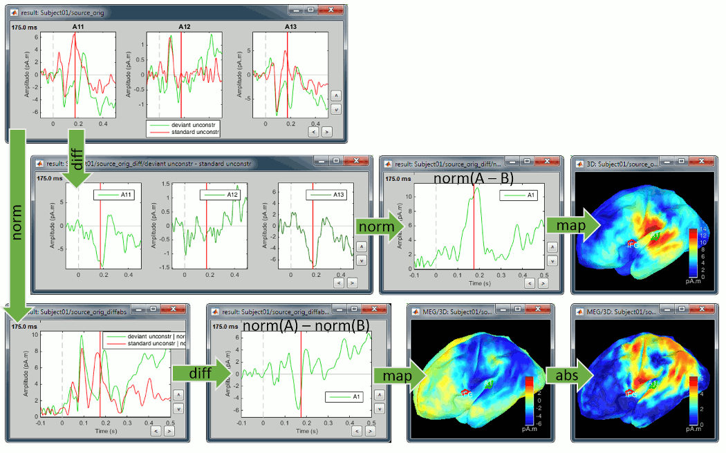
The exact same observations apply to the unconstrained sources, using the norm of the three orientations instead of the absolute values. X and Y represent the source vectors with three components each (x,y,z) for conditions A and B.
Norm(X-Y): This measure will detect vector differences between the two signals which can occur if the magnitude and/or orientation changes. It differs from (Norm(X)-Norm(Y)) in being sensitive to changes in apparent source orientation, but cannot differentiate increases from decreases in amplitude.
Norm(X)-Norm(Y): This is the unconstrained equivalent to |A|-|B|, i.e. it will produce a signed value that reflects increases or decreases in magnitude from A to B and should be interpreted similarly. Unlike Norm(X-Y) it is not sensitive to rotation of the source from A to B unless there is an accompanying amplitude change. But on the other hand, because the value is signed, we can differentiate between increases and decreases in amplitude.
Source normalization
The examples above only show minimum norm current density maps that haven't been normalized. The same logic applies to normalized source values, as long as you do not rectify the signals during the computation of the normalization.
As a reminder, you should normalize the source maps if you are intending to compare different subjects, it will help bringing them to the same range of values. The list below shows the valid operations for the Z-score normalization, but the same is applicable for dSPM, sLORETA and MNp.
Constrained sources:
Zscore(A) - Zscore(B): Correct amplitude, ambiguous sign.
abs(Zscore(A)) - abs(Zscore(B)): Ambiguous amplitude, meaningful sign.
Unconstrained sources:
norm(Zscore(A) - Zscore(B)): Correct amplitude, no sign.
norm(Zscore(A)) - norm(Zscore(B)): Ambiguous amplitude, meaningful sign.
Always avoid using the following measures:
- Z-score(abs(sources))
- Z-score(norm(sources))
Difference deviant-standard
Before running complicated statistical tests that will take hours of computation, you can start by checking what the difference of the average responses looks like. If in this difference you cannot observe the effects you are expecting, it's not worth moving forward with finer analysis: the recordings are not clean enough, you don't have enough data or your initial hypothesis is wrong.
Absolute difference: |A|-|B|
We are going to use the Process2 tab, at the bottom of the Brainstorm figure. It works exactly like the Process1 tab but with two lists of input files, referred to as FilesA (left) and FilesB (right).
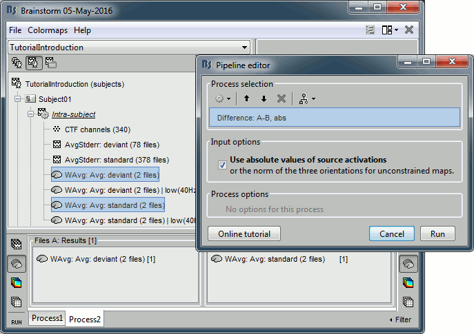
In Process2, drag and drop the non-normalized deviant average on the left (FilesA) and the non-normalized standard average on the right (FilesB).
Run the process "Difference > Difference A-B", select the option "Use absolute values".
Do run the computation now, we will add more steps.
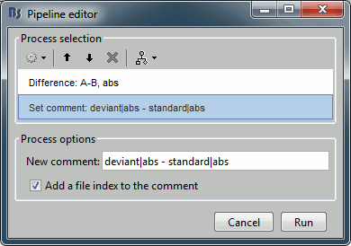
Add process: "File > Set comment", New comment = "deviant|abs - standard|abs"
Add process: "Standardize > Baseline normalization", Baseline=[-100,-1.7]ms, Method=Z-score
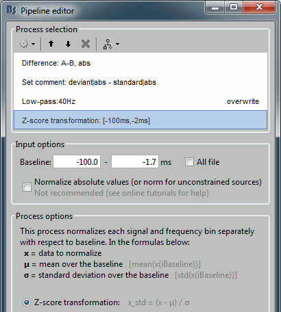
Add process: "Pre-process > Band-pass filter", Low-pass: 0-40Hz, Mirror, Overwrite.
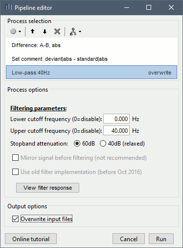
Run the script, then double-click on the filtered file and explore it in time. This is a cortex map, with positive and negative values. It should be displayed using a colormap that shows relative values (right-click > Colormap > Uncheck the option "Absolute values").
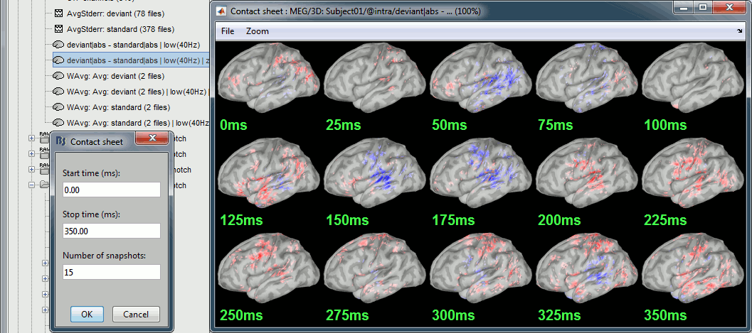
- We are looking at the rectified difference (abs(deviant)-abs(standard)) so positive/red regions indicate higher activity levels for the deviant beeps, and negative/blue regions higher activity for the standard beeps.
Before 50ms: The motor activity in the deviant is probably due to the previous stims.
50ms: Stronger auditory response in the standard condition.
MMN (125ms): Stronger response for the deviant (left temporal, left inferior frontal).
150ms: Stronger response in the auditory system for the standard condition.
175ms: Stronger response in the motor regions for the standard condition (motor inhibition).
After 200ms: Stronger response in the deviant condition (motor preparation and movement).
Plot the time series for scout A1L (relative and absolute values).
The relevant information here is the sign of the difference (option Values:Relative).

Relative difference: (A-B)
Recall the last analysis pipeline: menu File > Reload last pipeline.
In the process Difference: Unselect the option "Use absolute values".
In the process Set comment: Change the comment to "deviant - standard".
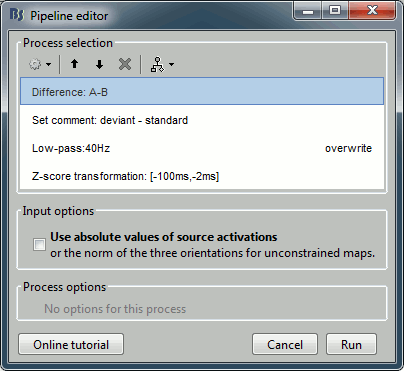
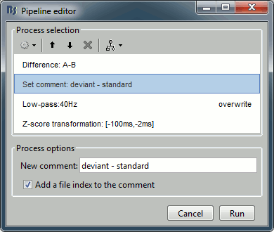
Run the script and open the filtered difference.
Change the colormap definition to show only positive values (right-click > Colormap: Stat2 > Uncheck: Absolute values) and use a different colormap ("hot" or "jet"). The sign of the relative difference is not meaningful, it depends mostly on the orientation of the dipoles on the cortex.
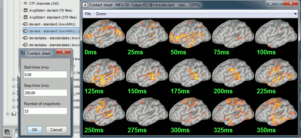
- We can see with much more contrast the areas and times where the two conditions are different, but we lose the ability to say which one is stronger. It is the measure we will use in most cases when computing statistical tests between conditions.
Plot the time series for scout A1L (relative values and absolute).
We observe the peak of difference where we were observing a zero with the absolute difference.

Difference of means
Another process can compute the average and the difference at the same time. We are going to compute the difference of all the trials from both runs at the sensor level. As discussed in the previous tutorials, this is usually not recommended because the subject might have moved between the runs. Averaging MEG recordings across runs is not accurate but can give a good first approximation, in order to make sure we are on the right tracks. It is acceptable here because the movements of the subjects are negligible between the two runs.
In Process2, select the following files:
Files A: all the deviant trials from both runs (~80 files)
Files B: all the standard trials from each run (~400 files).Select the process "File > Uniform number of files", with the default number of files and the option "Uniform". This will select the same number of files from FilesA and FilesB. The list with the larger number of files (FilesB) is sampled uniformly to get the same number of files on both sides.
This step is not necessary here, but it's a good time to illustrate it, in case you need it someday.
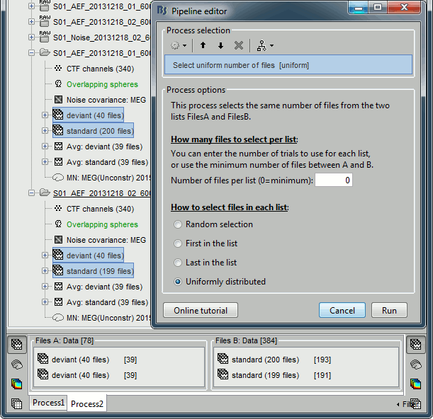
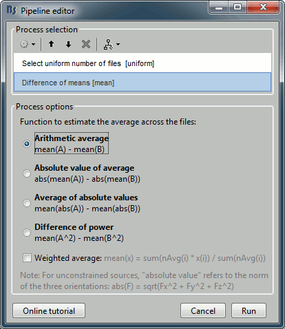
Add the process "Test > Difference of means", select the option "Arithmetic average".
The option "weighted average" has no importance because we are averaging only single trials.
Run the pipeline. Double-click on the new difference to display it. The difference does not show anymore the early responses (P50, P100) which are similar for the two conditions, but emphasizes the difference in the later process (MMN/P200 and P300).

Left: Average of 80 deviant trials.
Center: Average of 80 standard trials.
Right: Difference of the two, computed in this process.
Time-frequency
In the case of time-frequency maps there is no sign ambiguity of the values, so computing a difference is slightly simpler. There are two possible cases: difference between power maps or between normalized maps (eg. ERS/ERD).
Original time-frequency maps
- The power of the TF maps are only positive values, so you can simply compute the difference between the power maps, it will give you all the interesting information.
- Use the difference of the power: power(TF(A)) - power(TF(B))
- This is what you would use for computing statistics within a subject.
Normalized time-frequency maps
- The values represent deviations with respect with a baseline, they can be positive or negative. Therefore we are in the same configuration as with the sensor data.
- Use the difference of the normalized values: Normalize(power(TF(A))) - Normalize(power(TF(B)))
- This could be used for comparing visually two averages, or for statistics across subjects.
