Tutorial 9: Processes

The main window includes a graphical batching interface that directly benefits from the database explorer: files are organized as a tree of subjects and conditions, and simple drag-and-drop operations readily select files for subsequent batch processing. Most of the Brainstorm features are (or will be) available through this interface, including pre-processing of the recordings, averaging, time-frequency decompositions, and computing statistics. A full analysis pipeline can be created in a few minutes, saved in the user’s preferences and reloaded in one click, executed directly or exported as a Matlab script.

Selecting files to process

First thing to do is to define the files you are going to process. This is done easily by picking files or folders in the database explorer and droping them in the empty list of the Process1 tab.

1. Drag and drop the following nodes in the Process1 list: Right/ERF (recordings), Left (condition), and Subject01 (subject)
   
   

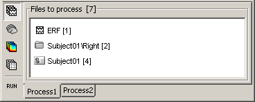
   • A number between brackets appear next to each node: it represents the number of data files that where found in each of them. The node ERF "contains" only itself (1), Subject01/Right contains ERF and Std files (2), and Subject01 contains 2 conditions x 2 recordings (4).
   • The total number of files, ie. the sum of all those values, appears in the title of the panel "Files to process [8]".

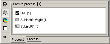
2. The buttons on the left side allow you to select what type of file you want to process: Recordings, sources, time-frequency, other. Now select the second button "Sources". All the counts are updated and now reflect the number of sources files that are found for each node
   
   

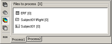
3. If you select the third button "Time-frequency", you would see "0" everywhere because there are no time-frequency decompositions in the database yet.
   
   

4. Now clear the list from all the files. You may either right-click on the list (popup menu Clear list), or select all the nodes (holding Shift or Crtl key) and then press the Delete key.

5. Select both files Left/ERF and Right/ERF in the tree (holding Ctrl key), and put the in Process list. We are going to apply some functions on those two files. You cannot distiguish them after they are dropped in the list, because they are both referred as "ERP". If at some point you need to know what is in the list, just leave you mouse over a node for a few seconds, and a tooltip would give you information about it. Just like in the database explorer.
   
   

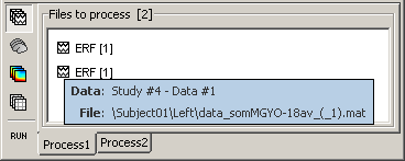
Creating a pipeline

List of processes

1. Click on Run. The Process selection window appears, with which you can create an analysis pipeline (ie. a list of process that are applyied on the selected files one after the other). The first button in the toolbar shows the list of processed that are currently available. If you click on a menu, it's added to the list.
   
   

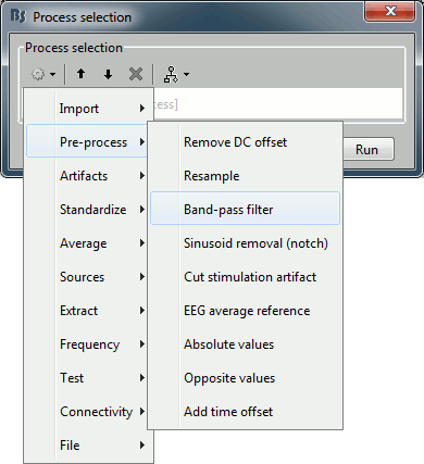
2. Some menus appear in grey (example: Normalize > Spatial smoothing). This means that they are not meant to be applied to the type of data that you have in input, or at the end of the current pipeline. The "spatial smoothing" process may only be run on source files.

3. When you select a process, a list of options specific to this process is shown in the window.

   • To delete a process: Select it and press the Delete key, or the big cross in the toolbar.

   • With the "up arrow" and "down arrow" buttons in the toolbar, you can move up/down a process in the pipeline.
4. Now add the following processes, and set their options:

   • Pre-process > Band-pass filter: 2Hz - 30Hz

     • In some processes, you can specify the type(s) of sensors on which you want to apply the process. This way you can for instance apply different filters on the EEG and the MEG, if you have both in the same files.

   • Extract > Extract time: 40.00ms - 49.60ms, overwrite initial file

     • This will extract from each file a small time window around the main response peak.
     • Selecting the overwrite option will replace the previous file (bandpass), with the output of this process (bandpass+extract). This option is usually unselected for the first process in the list, then selected automatically.

   • Average > Average over time: Overwrite initial file

     • Compute the average over this small time window.

   • Export > Export to Matlab variable: "avg45"

     • Reads the current file (time window averaged over time) and exports it in a variable in the Matlab workspace.
       
       

     

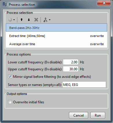
5. Save your pipeline: Click on the last button in the toolbar > Save > process_avg45.

Saving/exporting a pipeline

The last button in the the toolbar offers a list of menus to save, load and export the pipelines.

• 

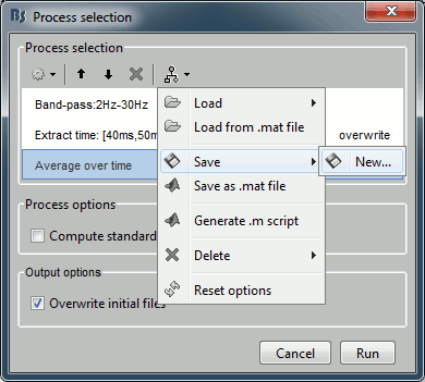
• Load: List of processes that are saved in the user preferences

• Load from file: Import a pipeline from a pipeline_...mat file (previously saved with the menu "Save as Matlab matrix")

• Save: Save the pipeline in the user preferencies, to be able to access it really fast after

• Save as Matlab matrix: Exports the pipeline for a Matlab structure in a .mat file. Allows different users to exchange their analysis pipelines (or a single user between different computers).

• Save as Matlab script: This option generates a human-readable Matlab script that can be re-used for other purposes or modified.

• Delete: Remove a pipeline that is saved in the user preferences.

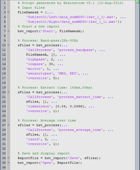
Here is the Matlab script that is generated automatically for this pipeline.

• 

Running a pipeline

1. Click on Ok, in the pipeline window. After a few seconds, you will see two new files in the database, and two messages in the Matlab command window. The file names have list of tags that where appended to represent all the processes that were applied to them.
   
   

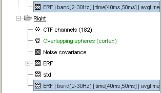
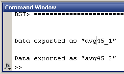
2. Quick reminder: the file history record all this information too (right-click > File > View file history), so you are free to rename those files in something shorter (example: "ERF_avg45").
   
   

3. Now double-click on the processed file in Right condition.
   • You see only horizontal lines. It is not a bug, it is because you averaged the data in time. There is no temporal dimension anymore.

   • Press Ctrl+T, to bring up a "2D sensor cap" view. It represents the average topography between 40ms and 50ms, filtered between 2Hz and 30Hz.
     
     

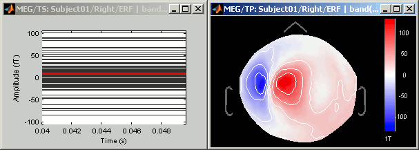
4. Now have a look to the output in the command window. Two variables where created, because there were two files in output "avg45_1" and "avg_45_2". Type "avg45_1" in the command window to see the fields in the structure:
   
   

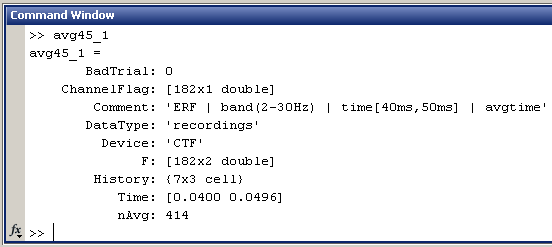
   • This is the exact same structure as the processed file in condition Left. All those fields where documented in the tutorial #2. Just notice the dimension of the recordings matrix F: [182 x 2], and the Time vector: [0.0400 0.0496]
   • In a general way, all the averages in time are represented in Brainstorm by two identical columns, one for the beginning and one for the end of the time window they represent.
5. Delete the two processed files, they are of no use after.

Another example: z-score and scouts

1. Load the two scouts LeftSS and RightSS saved in the previous tutorial.
2. Clear the files list and drag'n'drop "Subject01".
3. Select the "Results" button of the Process1 panel, it should indicate two files. Click on run.
4. Create the following pipeline:

   • Normalize > Z-score noise normalization: baseline = [-50ms,-1ms]

   • Extract > Scouts time series: select both scouts, and select "Concatenate output in one matrix"
     
     

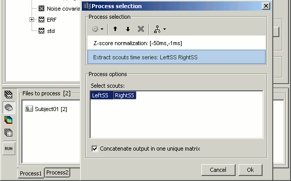
5. Run the pipeline. It creates three new files in the database:

6. 

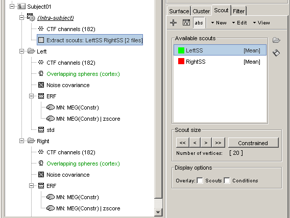
Let's have a detailed look at each of those files:

• Left / ERF / MN | zscore: Output of the zscore process for the Left sources

  • Double-click on it to display it. Display the original sources at the same time
    
    

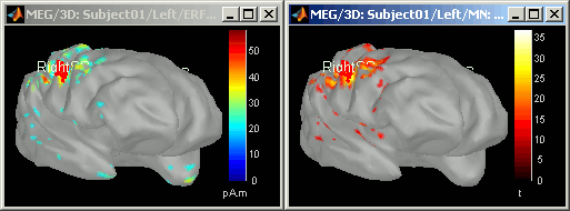
  • The z-score operation substracts the average and divide by the variance of the baseline. The goal is to give less importance to the sources that havea strong variability in the baseline, because they are considered as noise, and this way increase the visibility of the significant effects.
  • The maps look relatively similar in terms of localization, except that for the z-score, we do not observe any pattern of activity in the poles of the temporal lobes. The variance in those areas was high during the baseline, they have been "removed" by the z-score process.
  • Note that the units changed. The values of the z-score are without units (the minimum norm values where divided by their standard deviation)

• Right / ERF / MN | zscore: Output of the zscore process for the Right sources. Same thing.

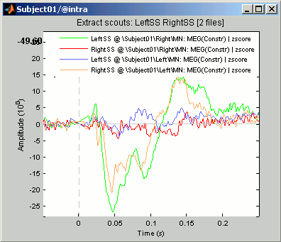
• Extract scouts: LeftSS RightSS [2 files]: Scouts times series for the two zscore files

  • This file was saved in a new node in the database: "Intra-subject". This is where are stored the results of processes that have in inputs files from different conditions within the same subject.
  • It contains the concatenated output of 2 scouts x 2 conditions, in one unique matrix. If we had not selected the "Concatenate" option, two files would have been saved, one in condition Left, one in condition Right.
  • This is a type of file that was not introduced yet in those tutorials. It is called simply "matrix", and may contain any type of data. Because we don't exactly know what they contain, the operations that can be performed on them are very limited.

• 

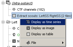
Available processes

Plugin structure

The available processes are organized in a plug-in structure. Any Matlab script that is added to the plug-in folder and has the right format will be automatically detected and made available in the GUI. This mechanism makes the contribution from other developers to Brainstorm very easy.

User processes