Review continuous recordings and edit markers

This tutorial describes how to review a continuous file and add time markers. It is based on a median nerve stimulation experiment recorded at the Montreal Neurological Institute in 2011 with a CTF MEG 275 system. The sample dataset contains 6 minutes of recordings at 1200Hz for one subject and includes 100 stimulations of each arm. The segmentation of the T1 MRI of the subject was performed using FreeSurfer.

Download and installation

• Requirements: You have already followed all the basic tutorials and you have a working copy of Brainstorm installed on your computer.

• Go to the Download page of this website, and dowload the file: sample_raw.zip

• Unzip it in a folder that is not in any of the Brainstorm folders (program folder or database folder). This is really important that you always keep your original data files in a separate folder: the program folder can be deleted when updating the software, and the contents of the database folder is supposed to be manipulated only by the program itself.
• Start Brainstorm (Matlab scripts or stand-alone version)

• Select the menu File > Create new protocol. Name it "TutorialRaw" and select the options: "No, use individual anatomy", "Yes, use one channel file per subject".

Import the anatomy

• Create a new subject Subject01

• In the anatomy view, right-click on the subject > Import FreeSurfer folder, and select the folder "sample_raw/Anatomy". This imports automatically all the available files in a segmentation folder generated with FreeSurfer, as illustrated in this page.

• Leave the default number of vertices of the cortex surface (15000)
• When asked to place the fiducials, you can use the file "sample_raw/Anatomy/fiducials.jpg".

• The picture shows the three head position coils used in the CTF systems. The positions of the fiducials were digitized with a Polhemus device at the middle of each of those coils. In the end, you should have the following MRI coordinates (+/- a few millimeters): NAS: x=126, y=215, z=138 LPA: x=58, y=136, z=121 RPA: x=197, y=138, z=118 AC: x=128, y=137, z=157 PC: x=128, y=113, z=157 IH: x=128, y=125, z=216 (anywhere on the midsagittal plane)

• Click on Save when you're done, and wait until the process is over. In the end, a figure shows the surfaces that were generated. Close it.
  
  

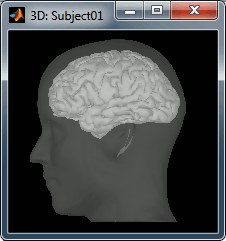
• Four files are now available as the anatomy of Subject01: a T1 MRI, a head surface, and two cortex surfaces (high and low resolution). The anatomy of the subject is ready.

Access the raw file

The basic tutorials you read before explain how to import recordings in the database: this operation creates a copy of all the data in Matlab .mat files in the Brainstorm database folders. You could process continuous recordings in the same way, but the .mat format has this limitation that the entire file has to be read even when you want to access just a portion of it. Long recordings usually cannot fit in memory and have to be split in small blocks of a few seconds, which makes it very difficult to review and process.

Brainstorm offers the possibility to visualize continuous MEG/EEG recordings in any of the supported file formats without having to fully "import" them. A link to the native file is created in the database, which can be then manipulated almost like the "imported" recording blocks. Only the description of the file is saved in the database, and when displaying it the values are read directly from the native file.

In addition, an interface allows to edit the time markers that are saved in the file. Those markers can then be used to import the recordings in the database (ie. to do the segmentation of the continous recordings in epochs/trials). Then the imported epochs/trials (hard copies in .mat format) can be pre-processed and averaged.

• Select the "Functional data (sorted by subject)" exploration mode (second button in the toolbar above the database explorer).

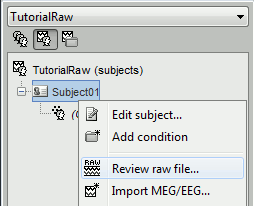
• Right-click on the subject node, and select: "Review raw file". Select the "MEG: CTF" file type, and pick the ds folder in "/sample_raw/Data".
  
  

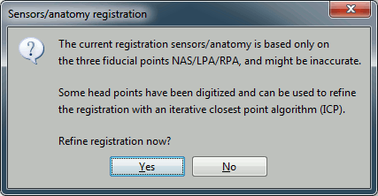
• Then you're asked if you want to "Refine the registration with the head points". This operation improves the initial MRI/MEG registration by fitting the head points digitized before the MEG acquisition on the scalp surface with an ICP algorithm. Answer yes. Even if the result is not perfect, it usually improves the positioning of the head in the MEG helmet.
  
  
  

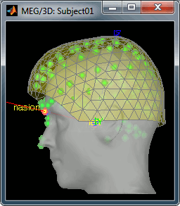
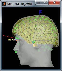
• Two new files appeared in the database explorer:
  
  

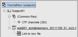
  • The channel file contains the definition of the sensors, exactly as when importing the files in the database with the "Import MEG/EEG" menu. It is saved in the folder (Common files), because the subject was created using the option "Yes, use one channel file per subject". Therefore, the same channel file will be used for all the folders of Subject01.

  • The node named "Link to raw file" contains all the information that was read from the continous file (file format, time vector, sampling frequency, events, bad channels, path to the original file, etc.), but no recordings. The MEG and EEG values recorded will be read directly from the native file.

Review the recordings

Open the file

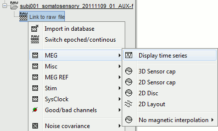
Right-click on the data file > MEG (all) > Display time series.

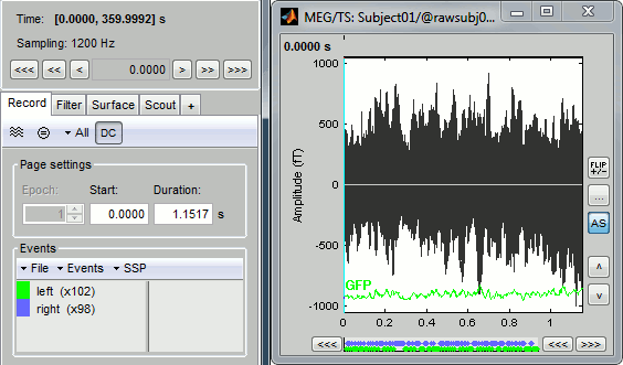
You can see a new tab "Event" and a figure showing the recordings.

Navigate in time

As described in the basic tutorials, you can set the current time by using either the time panel (buttons and text field), or the figure (click on the white or grey areas of the figure). But you can notice that only a few seconds are visible in the figure, while the time panel (top left of the previous figure), indicates that we have 360s of recordings. Only a small block of the continuous file has been loaded in memory. This small time window can be configured with the tab Event/Page settings, with the text boxes Start and Duration.

The time series figure is similar to the ones that were presented in the previous tutorials, with a few new elements. The navigation bar at the bottom represents the time of the entire raw file, where the events are also represented by dots. The '<<<' and '>>>' buttons are the same as the ones in the time panel, and jump to the previous/next segment in the file. Clicking on the bar or dragging the red cursor change the current time window as well.

Sensor selection

Let's switch to a nicer representation of the recordings time series: click on the "Display mode" button in the toolbar of the main Brainstorm window.

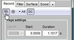
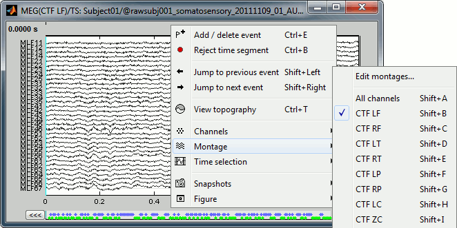
Now the traces are displayed in columns, but all the channels are displayed in the same figure, which makes it unreadable. Select a subset of channels by right-clicking on the figure > Display setup, or by using one of the keyboard shortcuts (Shift+A, B, C...). Default groups of sensors re available for some MEG systems, but you can also create your own groups of sensors with the menu "Edit selections".

Amplitude scale

In this display mode, the amplitude scale is represented on the right of the figure. You can adjust this vertical scale:

• Use the buttons "^" and "v" on the right side of the figure. The shortcuts for those buttons are indicated in the tooltips (leave the mouse for a short while over a button)

• Hold the Shift key and move the mouse wheel, or use the keys "+" and "-".

• Use the button "..." on the right side of the figure ("Set scale manually") to set the scale to a precise level.

When scrolling in time to a different page, the amplitude scale is by default kept. You can change this behavior to re-evaluate automatically an optimal scale each time you change the current time window. This option is called "Auto-scale amplitude" and is disabled by default. To activate it: click on the "AS" button on the right of the figure, or check the menu "Display > Auto-scale amplitude" in the Event tab.

Display options

• 

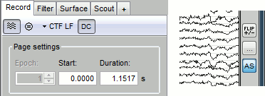
• Remove baseline: When selected, for each channel, the average value over the entire current time window is subtracted from the channel values. This means that if you change the length of the time window, the value that is removed from each channel may change. It doesn't make much sense to disable this option for unprocessed MEG recordings.

• Auto-scale amplitude: When selected, the vertical scale is adapted to the maximum value over the time window when the time window changes. When not selected: the vertical scales keeps its last value when you jump to another part of the file.

• Apply CTF compensation: Enable/disable the CTF noise correction based on the reference sensors, when it is not already applied in the file. In the current file, the CTF 3rd order gradient compensation is already applied, therefore this menu is not displayed.

Online filter

With the Filter tab, you can apply a band-pass filter to the recordings, or remove a set of specific frequencies (example: the 50Hz or 60Hz power lines contamination and their harmonics). The filters are applied only to the time window that is currently loaded; hence if the segment is too short for the required filters, the results could be inaccurate.

The option "Mirror signal before filtering" triples artifically the length of the signal with a mirror symmetry on each side, to avoid the strong edge effects that those filters can generate. Those online filters are not very accurate, they just provide a quick estimate for visualization only, the results are not saved anywhere. To filter properly the continuous files, please use the Process1 tab.

EEG Average reference

When reviewing EEG recordings, you can switch between the original values and the average reference by clicking on the "AVG REF" button in the toolbar of the main Brainstorm window. In this case, there is no EEG recorded in the file, so selecting this option or not does not change anything.

Average reference computation: at each time point, the average of all the electrodes values is subtracted from each electrode.

Events, markers, triggers

Lists of events

You probably noticed little green and blue dots on top of the recordings in the MEG figure. They represent the triggers of the electric stimulation. The stimulation computer sent those triggers simultaneously to the electric stimulator, which was converting them into electric pulses sent to the wrists of the subject, and to the acquisition computer, that was recording them together with the values of the MEG sensors.

All the temporal markers that are available in the file are listed in the Recordings section of the Event tab:

• on the left, the groups of events and the number of occurrence for each group (102 stimulations on the left, 98 on the right);
• on the right, all the occurrences of the selected event group, described by the time instant at which they occur.

Those two lists are interactive. If you click on a event group (left list), it shows the occurrences for the selected event in the right list. If you click on one particular event in the right list, the current time is set in the MEG figure to the selected event. If you click on a dot representing an event in the MEG figure, the corresponding event group and occurrence are selected in the Event tab.

Those "events" can represent either stimulation triggers that were recorded during the acquisition, or additional markers that were placed by the user during the analysis.

Adding events

First create a new group of events, define its name (test) and its color (red), with the "Events" menu in the Event tab:

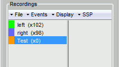
Then set the current time were you want to add a new Test even, by clicking on the figure (current time = where the vertical red line is). Select the group event "Test" and add a few occurrences with any of the three methods:

• In the Event tab: select the menu Events > Add event

• In the time series figure: right-click > Add event

• In the time series figure: press Ctrl + A

Now remove all the events occurrences, but not the group "Test":

• In the Event tab: select one or more event occurrences (mouse click + Shift or Control), and press the "Delete" key.

• In the time series figure: click on the event to delete (on the blue dot), and right-click > Delete event

• In the time series figure: click on the event to delete, and press Control + A

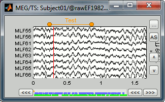
You can also use this interface to create events that have a temporal extension, ie. they last for more than one time sample. This is usually used to define bad/artifacted segments in the data.

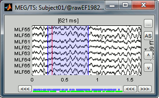
• In the time series window, select a time range (click + move) instead of just setting the current time.
• Note that you can click outside of the white area to select the time (on top of the figure), in order not to select channels instead of moving.
• Add an event (menus or Control+A): note the way it is represented in the figure and in the Event panel.
• The first occurrence you add in an event group defines the event type: single time point, or time range. You cannot mix different types of events in a group.

Custom shortcuts

Saving modifications

When you close the raw file viewer, or the last figure that shows a part of the raw file, the dataset is unloaded, the file is released and the memory is freed.

If you edited the events for this file, you would be asked whether to save the modifications or not. If you answer "Yes", the modifications to the events are only saved in the Brainstorm definition of the file, not in the raw file itself. So you would see your changes the next time you open the file with Brainstorm, but not if you open the raw file again with an external program.

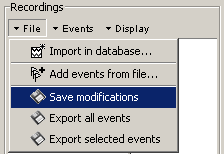
Note that events you edit are not saved automically until that moment. As you would do with any other type of work, save your work regularly, to limit the damages of a program or computer crash. In the Event tab, menu File > Save modifications.

Shortcut summary

Keyboard shortcuts

• Left / right arrows:

  • No other key: Change current time, sample by sample

  • With Control key: Jump to previous/next time segment (same as the "<<<" and ">>>" buttons)

  • With Shift key: Jump to next event of the selected group

  • On MacOS, these shortcuts are different: please read the tooltips from the buttons ">", ">>", and ">>>" in the time panel to get the appropriate shortcuts.

• Page-up / page-down:

  • Same as left/right arrows, but faster (10 samples at a time)

  • If epochs are defined in the file: Control + page-up/page-down jumps to the next/previous epoch.

• F3/Shift+F3: Jump to the next/previous epoch or page

• Plus / minus: Adjust the vertical scale of the time series

• Control + A: Add / delete event occurrence

• Control + T: Open a 2D topography window at the current time

• Shift + Letter: Changes the set of electrodes currently displayed in the figure (list available by right-clicking on the figure > Display setup > ...)

• Enter: Display the selected channels in a separate figure (selected channels = lines on which you clicked, that are shown in red)

• Escape: Un-select all the selected channels

• Delete: Mark the selected channels as bad

Mouse shortcuts

• Mouse click on a channel: Select the channel

• Mouse click: Change current time

• Mouse click + Shift: For the selection of the current time (do not select any sensor, even when clicking on a line)

• Mouse click + move: Select time range

• Mouse wheel: Zoom around current time

• Control + mouse wheel: Zoom vertically

• Shift + mouse wheel: Adjust the vertical scale of the time series

• Right-click: Display popup menu

• Right-click + move: Move in a zoomed figure

• Double click: Restore initial zoom settings (but do not restore the vertical scale of the time series)

Other views

Topography views

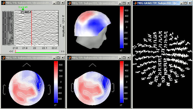
Exactly as introduced in the ?tutorial #4 "Exploring the recordings", you can display a variety of 2D/3D mappings of those recordings. Right-click on the node "Link to raw file" > MEG (all) > ...

Cortical sources

As presented in tutorial #5 to #7, you can compute successively for this raw file: a head model, a noise covariance matrix, and an inverse model.

• Head model: The goal of this tutorial is only to illustrate what you can do with the raw file viewer in Brainstorm, not to localize anything for real. Keep all the default options for the head model computation.

• Noise covariance matrix: Set as the baseline section the entire window before the first electric stimuation (the first occurrence of Event #5): [27.799, 41.170] seconds. Leave the other options to the default values.

• Sources: Keep the default options for the minimum norm method (wMNE).

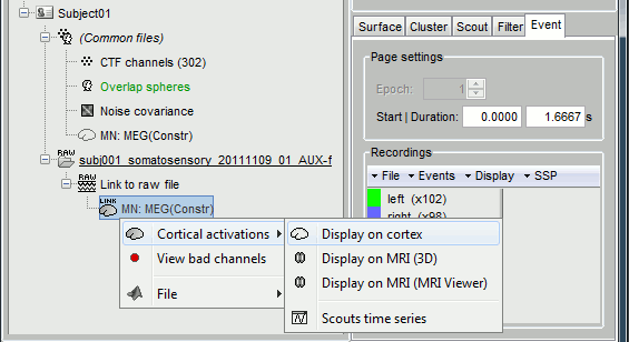
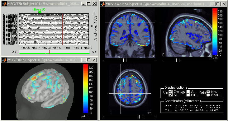
At the end you can see three new files in the database. Right-click on the sources and try the different visualization menus.

Important: Remember that you probably still have the online filter on; the band-pass options you specify in the Filter panel are kept until you close Brainstorm.