|
Size: 19183
Comment:
|
Size: 19293
Comment:
|
| Deletions are marked like this. | Additions are marked like this. |
| Line 1: | Line 1: |
| '''[WARNING: This page is part of the old tutorials, please refer to the [[Tutorials|new documentation]]]'''<<BR>><<BR>><<BR>> |
|
| Line 2: | Line 4: |
| ''Authors: Francois Tadel, John C Mosher, Sylvain Baillet'' | ''Authors: Francois Tadel, John C Mosher, Richard Leahy, Sylvain Baillet'' |
| Line 11: | Line 13: |
| The scouts are saved automatically in the surface file from which they are created, and they are loaded and displayed automatically each time the surface is loaded. | The scouts are automatically saved in the surface file from which they are created, and they are loaded and automatically displayed each time the surface is loaded. |
| Line 13: | Line 15: |
| An ''atlas'' designates in this context a list of scouts. It is possible to have one or more ''atlases'' saved for each file, that can be generated automatically from Brainstorm, from an external software like !FreeSurfer (see [[Tutorials/LabelFreeSurfer|this page]]), or created manually scout by scout. All the cortex surfaces contain by default an empty atlas called "User scouts", for the user to create new regions of interest. | An ''atlas'' designates in this context a list of scouts. It is possible to have one or more ''atlases'' saved for each file, that can be automatically generated from Brainstorm, from an external software like FreeSurfer (see [[Tutorials/LabelFreeSurfer|this page]]), or created manually scout by scout. All the cortex surfaces contain by default an empty atlas called "User scouts", for the user to create new regions of interest. |
| Line 19: | Line 21: |
| 1. Switch to the ''Scout'' tab, click on the first button in the toolbar (the big cross), and then click in the middle of the red stain in left hemisphere in the 3D figure (rotate and zoom before if necessary). A small dot with the label "1" appears where you clicked. Your first scout is created in the ''User scouts'' atlas, and contains only one vertex for the moment. <<BR>><<BR>> {{attachment:firstScout.gif}} | 1. Switch to the ''Scout'' tab, click on the first button in the toolbar (the big cross), and then click in the middle of the red area in left hemisphere in the 3D figure (rotate and zoom before if necessary). A small dot with the label "1" appears where you clicked. Your first scout is created in the ''User scouts'' atlas, and contains only one vertex for the moment. <<BR>><<BR>> {{attachment:firstScout.gif}} |
| Line 24: | Line 26: |
| In this case, the source is so focal that we could even use only the first vertex we selected to represent this area. But most of the time, the aim of a scout is to get the average activity over a larger region; so for the example, let's grow this scout. The buttons in in the ''Scout size'' panel offer basic operations to define the scout extension. | In this case, the source is so focal that we could even use only the first vertex we selected to represent this area. But most of the time, the aim of a scout is to get the average activity over a larger region; so for the example, let's grow this scout. The buttons in the ''Scout size'' panel offer basic operations to define the scout extension. |
| Line 96: | Line 98: |
| We are going to create an other scout for the other condition: the stimulation of the '''left thumb'''. | We are going to create another scout for the other condition: the stimulation of the '''left thumb'''. |
| Line 103: | Line 105: |
| 1. Create a new scout at this point. Name it ''RightSS'', for Right !SomatoSensory cortex. | 1. Create a new scout at this point. Name it ''RightSS'', for Right SomatoSensory cortex. |
| Line 130: | Line 132: |
| * '''Load atlas''': Load ROIs or a cortical parcellation coming from !FreeSurfer or !BrainSuite as a new atlas. | * '''Load atlas''': Load ROIs or a cortical parcellation coming from FreeSurfer or BrainSuite as a new atlas. |
| Line 146: | Line 148: |
| * '''Surface clustering''': Create a parcellation of the cortex surface and saves it as a new atlas. Can be useful for studying the connectivity between different regions of the brain. Only the "Random" clustering is currently available. Experimental features. | * '''Surface clustering''': Create a parcellation of the cortex surface and saves it as a new atlas. Can be useful for studying the connectivity between different regions of the brain. Only the "Homogeneous parcellation" options are currently reliable. |
| Line 169: | Line 171: |
| * '''Edit surface''': Create a new surface containing only the desired parts (remove or keep only the selected scouts). This is useful for instance for selecting one sub-cortical region from the Aseg !FreeSurfer atlas (see the [[Tutorials/LabelFreeSurfer|FreeSurfer tutorial]]). | * '''Edit surface''': Create a new surface containing only the desired parts (remove or keep only the selected scouts). This is useful for instance for selecting one sub-cortical region from the Aseg FreeSurfer atlas (see the [[Tutorials/LabelFreeSurfer|FreeSurfer tutorial]]). |
| Line 180: | Line 182: |
| A scout is defined by its name, and it has several properties: a list of vertices and an aggregating function. Those are usually enough to explore the activity at the cortex level the way we did it in those tutorials. An extra property can be defined on the scout: the explicit classification in a brain region. This property is used only in more advanced functional connectivity analysis, for the representation of the NxN connection graphs. It is introduced here for reference purpose. | A scout is defined by its name, and it has several properties: a list of vertices and an aggregating function. These are usually enough to explore the activity at the cortex level the way we did it in these tutorials. An extra property can be defined on the scout: the explicit classification in a brain region. This property is used only in more advanced functional connectivity analysis, for the representation of the NxN connection graphs. It is introduced here for reference purpose. |
| Line 186: | Line 188: |
| When set, the region string is shown before the scout name in the list, representing only the defined levels. It doesn't shown the letters U for "undefined", therefore the scouts you create manually, that are by default set to "UU", do not show any extra string. | When set, the region string is shown before the scout name in the list, representing only the defined levels. It doesn't show the letters U for "undefined", therefore the scouts you create manually, that are by default set to "UU", do not show any extra string. |
| Line 190: | Line 192: |
| == Feedback == <<EmbedContent(http://neuroimage.usc.edu/brainstorm3_register/get_feedback.php?Tutorials/TutScouts)>> |
|
| Line 195: | Line 194: |
<<EmbedContent(http://neuroimage.usc.edu/brainstorm3_register/get_feedback.php?Tutorials/TutScouts)>> |
[WARNING: This page is part of the old tutorials, please refer to the new documentation]
Tutorial 9: Scouts
Authors: Francois Tadel, John C Mosher, Richard Leahy, Sylvain Baillet
In Brainstorm jargon, a scout is a region of interest (ROI) defined on the cortical surface: a subset of vertices of this surface. This document explains how to create one or several scouts, use them to retrieve the activity in specific brain regions, and compare between conditions.
Contents
Creating a scout
Almost all the features related to the scouts manipulation are accessible in the Scout tab in the main Brainstorm window. We are going to use this panel to create a scout that includes the cortical area that we observed in the previous tutorial: the one that responds to the stimulation of the right thumb.
The scouts are automatically saved in the surface file from which they are created, and they are loaded and automatically displayed each time the surface is loaded.
An atlas designates in this context a list of scouts. It is possible to have one or more atlases saved for each file, that can be automatically generated from Brainstorm, from an external software like FreeSurfer (see this page), or created manually scout by scout. All the cortex surfaces contain by default an empty atlas called "User scouts", for the user to create new regions of interest.
First vertex (seed)
Select the protocol TutorialCTF, and display the times series for Subject01 / Right / ERF (double-click).
- Display the associated sources (try it from the time series figure: Ctrl+S, or figure popup menu)
- Go to 48ms, and set the data threshold around 90%.
Switch to the Scout tab, click on the first button in the toolbar (the big cross), and then click in the middle of the red area in left hemisphere in the 3D figure (rotate and zoom before if necessary). A small dot with the label "1" appears where you clicked. Your first scout is created in the User scouts atlas, and contains only one vertex for the moment.
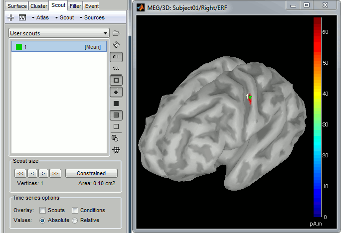
Rename the scout into "LeftSS", for left somatosensory cortex: double-click on it in the Available scouts list, or scouts menu Edit > Rename.
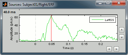
Click on the second button in the Scouts panel toolbar, tooltip: Display scouts time series. And you will get the time course of this particular source for the whole time window (-50ms to 250ms).
Growing a scout
In this case, the source is so focal that we could even use only the first vertex we selected to represent this area. But most of the time, the aim of a scout is to get the average activity over a larger region; so for the example, let's grow this scout. The buttons in the Scout size panel offer basic operations to define the scout extension.
'>': Add the closest vertex (with respect to the seed) to the current scout.
'<': Remove the furthest vertex (with respect to the seed) from the current scout.
'>>': Grow scout in all directions
'<<': Shrink scout in all directions
'Constrained': If this button is pressed, only the vertices that have a sources value above the threshold will be added to the scout (its growth will be limited to the red patch on the surface).
Add vertex manually: Select the Select point button, then select again the "LeftSS" scout. When you click on a vertex on the surface, it is added to the selected scout.
Remove vertex manually: Same as previously, but holding the SHIFT key at the same time.
Now: add about 15-20 vertices with button '>>', not in Constrained mode, and display the scout values again. You can notice that the overall shape is the same as the scout with only one vertex, but the amplitudes are much lower. This is because the time series of all the sources in this scout have been averaged. And as we averaged the maximum values with lower values, the result is lower.

Display options
In the toolbar on the right side of scouts tab, you can find a list display options. Leave your mouse over it for a few seconds to get a description of each of them.
 Load Atlas
  Save selected scouts
  Show all the scouts
  Show only the selected scouts
 - If both previous buttons are unselected: no scouts are displayed in the 3D figure. It can be interesting to hide all the scouts if you are working with atlases on hi-resolution surfaces and if it takes to long to open a surface.
 Show / hide the contour line
  Show / hide the scouts labels
  Scout patch: Opaque
  Scout patch: Transparent
  Scout patch: None
  Display the color of the region instead of the scout color (only for anatomical atlases)
  Center MRI on scout (opens the MRI viewer and set the position to the current scout)
Scout function
How are the scouts time series calculated? For the scout LeftSS we have 15 signals, coming from 15 different dipoles with different orientations, that are combined into one unique signal. In the list of available scouts, you can see the indication "[mean]" next to the name of the scout. It represents the name of the function that is used for combined all the time series into one. This function can be changed individually for each scout, with the menu Scout > Set function in the Scout tab.
List of the functions
Here is a description of the different options. In the case of unconstrained sources (3 signals for each vertex, one for each orientation), the function is applied separately for each orientation and produces 3 time series instead of one. For more details, see the code of bst_scout_value.m.
Mean: Average all the signals
PCA: Take the first mode of the PCA decomposition of all the signals.
Fast PCA: Same as PCA function, but computes the first PCA decomposition based only on a subset of the most powerful signals. It gives very similar results, but its computation is much faster for scouts that group a large number of dipoles (>50).
Mean(norm): Average the absolute values of all the signals
Max: For each time point, get the maximum across all the vertices [signed maximum in amplitude value: m = max(abs(signal)), scout = sign(signal(m)) * m]
Power: Average the power of all the signals (signal^2)
All: Do not apply any operation on the scouts signals, and display the time series of all the sources at the same time.
"Absolute" display option
As said in the previous tutorial, the minimum norm current amplitudes can positive or negative. Which means that the values of the scouts, depending on the function that is used, may be positive or negative too. Most of the time we are interested in visualizing the absolute values of the scouts time series, to compare the activation level in different conditions or subjects.
For this purpose, at the bottom of the Scout tab, you can choose to display either Absolute or Relative values. The effect of this options depends if you are processing sources with constrained (1 signal per vertex) or unconstrained (3 signals per vertex) orientations:
Constrained: Applies the scout function sfunction to all the N sources time series, and then apply or not an absolute value
Absolute: abs(sfunction(sources))
Relative: sfunction(sources)
Unconstrained: Applies the scout function sfunction to the N sources time series for each orientation (x,y,z) separately, and then returns either the norm of the 3 orientations, or each orientation separately
Absolute: Returns one time series:
sqrt( sfunction(sources_x).^2 + sfunction(sources_y).^2 + sfunction(sources_z).^2)Relative: Returns three time series:
sfunction(sources_x), sfunction(sources_y), sfunction(sources_z)
Change the selection to Relative and display again the activation of scout LeftSS for condition Right.
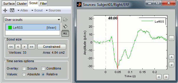
The effect of the function depends if you are processing sources with constrained (1 signal per vertex) or unconstrained (3 signals per vertex) orientations.
Note that it is a display option, it is not saved in the scouts themselves. It is used ONLY when displaying the scouts time series with the "Display" button of the Scout tab. In all other cases, like the extraction of the scouts values from a script, this relative/absolute option is going to be ignored.
Testing the functions
Now, leave this Relative option selected for testing all the scouts functions one by one.
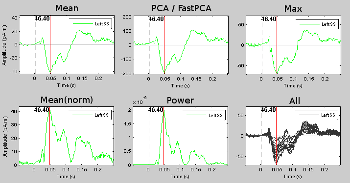
Select again the "Absolute" display again, and keep it for the rest of the tutorial.
Multiple scouts
We are going to create another scout for the other condition: the stimulation of the left thumb.
- Close all figures (toolbar button).
Display the times series for Subject01 / Left / ERF (double-click).
- Display the associated sources (Ctrl+S).
- Go to the main response peak (46 ms).
- Adjust the threshold value to get only a very focal point (about 60%).
Create a new scout at this point. Name it RightSS, for Right SomatoSensory cortex.
Grow it to the same number of vertices as the LeftSS scout (about 15 vertices).
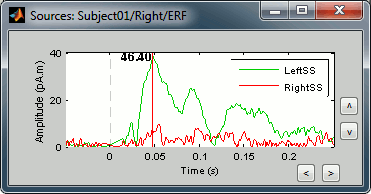
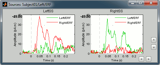
Select both scouts (Ctrl+click) and click on Display scouts time series button (second button in toolbar).
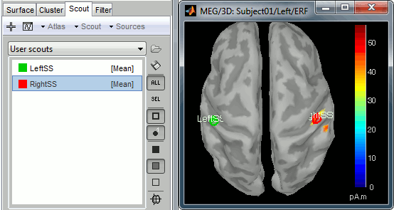
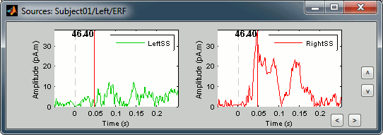
You can display the values of the two scouts on the same graph. Check the Overlay > Scouts checkbox in the Scout tab, and hit the Display scouts time series button again.

You can observe something that we expected: the activity in the right somatosensory cortex is much higher than in the left somatosensory cortex for a stimulation of the left thumb.
Display scouts from the database explorer
You have to display the sources on the cortex to create the scouts. But once they are created, you can directly display the scouts time series from the tree. It means that you can quickly compare the values for a scout between many different conditions without having to open them all.
- Close all the figures (button in toolbar)
- Select the options "values: absolute" and "overlay: scouts"
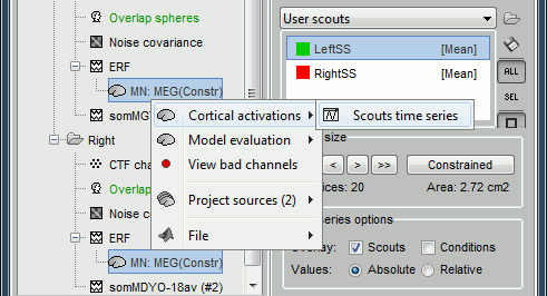
Right-click on Right / ERF / MN > Cortical activations > Scouts time series.
By default it shows all the scouts that are available in the current atlas.
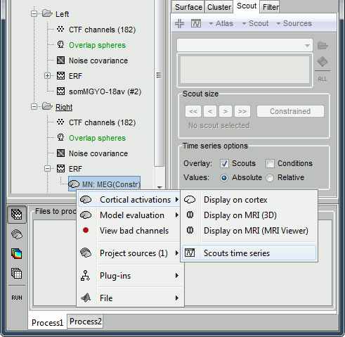
Note that if a surface is loaded, and at least one scout selected in the Scout tab, this popup menu would display only the selected scouts.
You can also display the scout values for many source files at the same time. Now keep the previous figure opened, so you have access to the scouts list in the Scout tab. Select only the LeftSS scout. In the database explorer, select at the same time the source files from condition Left and Right > right-click > Cortical activations > Scouts time series.
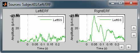
You can superimpose the two traces from the two experimental conditions by selecting the Overlay > Conditions checkbox in Scout panel. Select again the two files > Right click > Scouts time series. We see now the activation of the LeftSS scout for the stimulation of both thumbs.
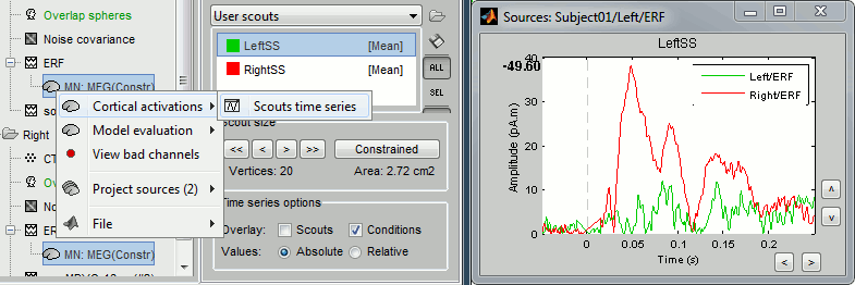
This menu "Scouts time series" is present at all the levels in the tree. Try right-clicking on Subject01 > Scouts time series.
If you select a node in the database tree and click on the Display scouts time series button in the Scout tab, it would have exactly the same effect.
Try selecting both scouts in the list, select Subject01 in the tree, overlay / conditions, and then click on this button. You will see the response for each scout in both conditions.
Scout toolbar and menus
Let's spend a few minutes to explore all the menus in the Scout tab. Don't hesitate to click on all of them, it's the best way to remember what they do.
Menu: Atlas
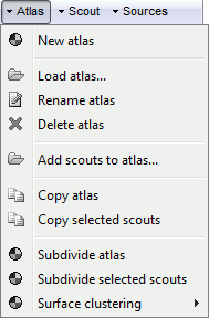
New atlas: Create a new empty atlas.
Load atlas: Load ROIs or a cortical parcellation coming from FreeSurfer or BrainSuite as a new atlas.
Rename atlas: Change the name that appears in the atlas list to refer to the selected atlas
Delete atlas: Delete the atlas and all the scouts in contains. The "User scouts" entry cannot be deleted.
Add scouts to atlas: Load ROIs or a cortical parcellation and add them to the current atlas.
Copy atlas: Duplicates an atlas and all the scouts
Copy selected scouts: Copy the selected scouts, and paste them in a new empty atlas.
Subdivide atlas: Splits all the scouts of the current atlas in smaller ROIs. Available options:
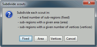
Subdivide selected scouts: Same thing, but processes only the selected scouts.
Surface clustering: Create a parcellation of the cortex surface and saves it as a new atlas. Can be useful for studying the connectivity between different regions of the brain. Only the "Homogeneous parcellation" options are currently reliable.
Menu: Scout
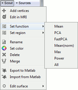
Add vertices: The user can select some points on the cortex surface and add them to the scout.
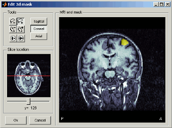
Equivalent: Click on Select point (first toolbar button), then select the scout in list, and select 3d points.Edit in MRI: Open an interface to edit the select scout as a 3D ROI, slice by slice.
- Define the 3D mask using the drawing tools (read the tooltips of the buttons for help).
- Adjust the MRI contrast with right-click+move on the MRI image.
- Move through the slices with the mouse wheel, the small image on the left, or the slider.
Warning: Only the vertices contained in the 3D mask are kept, all the volume information is lost. It means that the mask you intendend to draw might be very different from what you get as a scout at the end...
Set function: Set the scout function for the selected scouts.
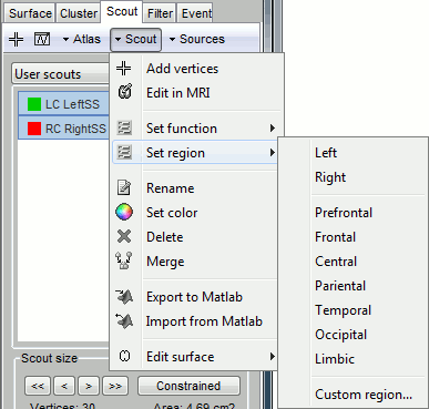
Set region: Set the cortical region for the selected scouts. This information is useful when representing functional connectivity graphs.
Rename: Rename the selected scout. Shortcut: double-click.
Set color: Change the display color of scout patch in 3D figures.
Delete: Delete selected scouts. Shortcut: Delete key
Merge: Join two or more selected scouts.
Export to Matlab: Export the structures of the selected scouts to the Matlab environment, and makes them accessible from the command window. This menu can be useful to get quickly the list of vertices in the scout.
Import from Matlab: Import scouts structures that you modified manually from your Matlab command window directly as new scouts.
Edit surface: Create a new surface containing only the desired parts (remove or keep only the selected scouts). This is useful for instance for selecting one sub-cortical region from the Aseg FreeSurfer atlas (see the FreeSurfer tutorial).
Menu: Sources
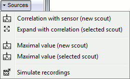
Simulate recordings: Multiply the selected scouts with the forward model. Simulate the scalp data that would be recorded if only the selected cortex region was activated; all the other sources are set to zero. Create a new data file in the database.
If no scout selected: simulate recordings produced by the activity of the entire cortex.Correlation with sensor: Create a new scout with all the sources that are strongly correlated with a given sensor.
Expand with correlation: Computes the correlation between the values for the scout's seed (first point) and all the other sources. The sources that have correlation coefficient superior to a given threshold are added to the scout. Correlation is computed with the Matlab corrcoef function.
Maximal value (new scout): Find the vertex with the maximal intensity at the current time, and create a scout centered on it.
Maximal value (selected scout): Move the scout's seed to the source that has the maximum amplitude in the scout, at the current time.
Scout region
A scout is defined by its name, and it has several properties: a list of vertices and an aggregating function. These are usually enough to explore the activity at the cortex level the way we did it in these tutorials. An extra property can be defined on the scout: the explicit classification in a brain region. This property is used only in more advanced functional connectivity analysis, for the representation of the NxN connection graphs. It is introduced here for reference purpose.
A brain region in Brainstorm is following a hierarchy with three levels: hemisphere / lobe / sub-region. The definition at each level is optional: a region can be classified only at the hemisphere level, or at the hemisphere+lobe level, or none of them. It depends on level or hierarchy you are interested in to explore the connectivity graphs.
The region for a scout can be set with the Scout > Set region menus, and is encoded in a string that contains at least 2 characters: "HLxxx". H represents the hemisphere (L,R,U), L stands for the lobe (F,PF,C,P,T,O,L,U), and xxx for the sub-region name (optional). For both the hemisphere and the lobe, the value "U" stands for "Undefined", meaning that the classification is simply not set. The menu Set region>Custom region... lets you edit this string directly. The menu Set region>Undefined sets the region string to "UU" (undefined hemisphere, undefined lobe).
When set, the region string is shown before the scout name in the list, representing only the defined levels. It doesn't show the letters U for "undefined", therefore the scouts you create manually, that are by default set to "UU", do not show any extra string.
Next
Next step, the ?graphical batching interface.

