Differences between revisions 2 and 79 (spanning 77 versions)

MEG visual tutorial: Group analysis

Authors: Francois Tadel, Elizabeth Bock.

The aim of this tutorial is to reproduce in the Brainstorm environment the analysis described in the SPM tutorial "Multimodal, Multisubject data fusion". The data processed here consists in simultaneous MEG/EEG recordings of 19 subjects performing simple visual task on a large number of famous, unfamiliar and scrambled faces. This tutorial follows another page that explains how to process one single subject in details.

Contents

License
Download and installation
Overview of the analysis
1. Coregistration of the acquisition runs
2. Objectives [TODO]
Subject averages: Famous, Unfamiliar, Scrambled
Subject averages: Faces
Subject averages: Within-subject differences
1. Sources: Faces - Scrambled
2. Sources: Famous - Unfamiliar
Subject averages: Filter and normalize
Subject averages: Screen captures
Group analysis: MEG/EEG
Group analysis: Sources
Scripting

License

This dataset was obtained from the OpenfMRI project (http://www.openfmri.org), accession #ds117. It is made available under the Creative Commons Attribution 4.0 International Public License. Please cite the following reference if you use these data:
Wakeman DG, Henson RN, A multi-subject, multi-modal human neuroimaging dataset, Scientific Data (2015)

Any questions, please contact: rik.henson@mrc-cbu.cam.ac.uk

Download and installation

First, make sure you have enough space on your hard drive, at least 30Gb:

The Brainstorm database with all the data imported, downloaded from this website: 20Gb
The same database after this tutorial: 30Gb

You can follow this tutorial after processing the recordings for the 19 subjects (6 runs per subject) as illustrated in the single subject tutorial. Otherwise, we provide a Brainstorm protocol that includes all the imported data, downsampled at 275Hz:

Go to the Download page, download the file TutorialGroup.zip (20Gb).
Unzip this file in your Brainstorm database folder (brainstorm_db).
In Brainstorm, menu File > Load protocol > Load from folder > Select brainstorm_db/TutorialGroup

The database you need in order to follow this tutorial should contain the following:

The individual anatomy imported from FreeSurfer or BrainSuite for each subject (19 subjects).
The sensor level averages (MEG+EEG) for each run (downsampled to 275Hz or not).
The forward model, noise covariance and inverse models for each subject and each run.
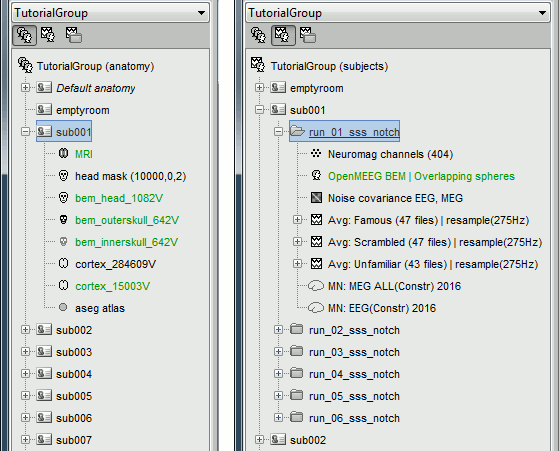
This protocol TutorialGroup is produced from the single subject protocol TutorialVisual with the script: brainstorm3/toolbox/script/tutorial_visual_copy.m

1 function tutorial_visual_copy(ProtocolNameSingle, ProtocolNameGroup, reports_dir) 2 % TUTORIAL_VISUAL_COPY: Copy the subject averages for the Brainstorm/SPM group tutorial into a new protocol (BIDS VERSION) 3 % 4 % ONLINE TUTORIALS: 5 % - https://neuroimage.usc.edu/brainstorm/Tutorials/VisualSingle 6 % - https://neuroimage.usc.edu/brainstorm/Tutorials/VisualGroup 7 % 8 % INPUTS: 9 % - ProtocolNameSingle : Name of the protocol created with all the data imported (TutorialVisual) 10 % - ProtocolNameGroup : Name of the protocol with just the averages, downsampled to 275Hz (TutorialGroup) 11 % - reports_dir : If defined, exports all the reports as HTML to this folder 12 13 % @============================================================================= 14 % This function is part of the Brainstorm software: 15 % https://neuroimage.usc.edu/brainstorm 16 % 17 % Copyright (c) University of Southern California & McGill University 18 % This software is distributed under the terms of the GNU General Public License 19 % as published by the Free Software Foundation. Further details on the GPLv3 20 % license can be found at http://www.gnu.org/copyleft/gpl.html. 21 % 22 % FOR RESEARCH PURPOSES ONLY. THE SOFTWARE IS PROVIDED "AS IS," AND THE 23 % UNIVERSITY OF SOUTHERN CALIFORNIA AND ITS COLLABORATORS DO NOT MAKE ANY 24 % WARRANTY, EXPRESS OR IMPLIED, INCLUDING BUT NOT LIMITED TO WARRANTIES OF 25 % MERCHANTABILITY AND FITNESS FOR A PARTICULAR PURPOSE, NOR DO THEY ASSUME ANY 26 % LIABILITY OR RESPONSIBILITY FOR THE USE OF THIS SOFTWARE. 27 % 28 % For more information type "brainstorm license" at command prompt. 29 % =============================================================================@ 30 % 31 % Author: Francois Tadel, Elizabeth Bock, 2016-2018 32 33 % ===== CHECK PROTOCOLS ===== 34 % Start brainstorm without the GUI 35 if ~brainstorm('status') 36 brainstorm nogui 37 end 38 % Output folder for reports 39 if (nargin < 3) || isempty(reports_dir) || ~isdir(reports_dir) 40 reports_dir = []; 41 end 42 % You have to specify the folder in which the tutorial dataset is unzipped 43 if (nargin < 2) || isempty(ProtocolNameSingle) || isempty(ProtocolNameGroup) 44 ProtocolNameSingle = 'TutorialVisual'; 45 ProtocolNameGroup = 'TutorialGroup'; 46 end 47 48 % Output protocol: Delete existing protocol 49 gui_brainstorm('DeleteProtocol', ProtocolNameGroup); 50 % Output protocol: Create new protocol 51 iProtocolGroup = gui_brainstorm('CreateProtocol', ProtocolNameGroup, 0, 0); 52 % Output protocol: Get protocol information 53 ProtocolInfoGroup = bst_get('ProtocolInfo'); 54 55 % Input protocol: Check that it exists 56 iProtocolSingle = bst_get('Protocol', ProtocolNameSingle); 57 if isempty(iProtocolSingle) 58 error(['Unknown protocol: ' ProtocolNameSingle]); 59 end 60 % Select input protocol 61 gui_brainstorm('SetCurrentProtocol', iProtocolSingle); 62 % Input protocol: Get protocol information 63 ProtocolInfoSingle = bst_get('ProtocolInfo'); 64 65 66 % ===== COPY ONLY GOOD SUBJECTS ===== 67 % Start a new report (one report per subject) 68 bst_report('Start'); 69 % Loop on subjects 70 for iSubj = 1:16 71 % Subject folders 72 SubjectName = sprintf('sub-%02d', iSubj); 73 AnatSrc = bst_fullfile(ProtocolInfoSingle.SUBJECTS, SubjectName); 74 DataSrc = bst_fullfile(ProtocolInfoSingle.STUDIES, SubjectName); 75 AnatDest = bst_fullfile(ProtocolInfoGroup.SUBJECTS, SubjectName); 76 DataDest = bst_fullfile(ProtocolInfoGroup.STUDIES, SubjectName); 77 % If subject folder doesn't exist: skip 78 if ~file_exist(AnatSrc) || ~file_exist(DataSrc) 79 disp(['Subject "' SubjectName '" does not exist or is incomplete.']); 80 continue; 81 end 82 % Copy anatomy files 83 mkdir(AnatDest); 84 disp(['Copying: ' AnatSrc ' to ' AnatDest '...']); 85 file_copy(bst_fullfile(AnatSrc, '*.mat'), AnatDest); 86 % Copy analysis folders 87 mkdir(bst_fullfile(DataDest, '@default_study')); 88 mkdir(bst_fullfile(DataDest, '@intra')); 89 disp(['Copying: ' DataSrc ' to ' DataDest '...']); 90 file_copy(bst_fullfile(DataSrc, '@default_study', '*.mat'), bst_fullfile(DataDest, '@default_study')); 91 file_copy(bst_fullfile(DataSrc, '@intra', '*.mat'), bst_fullfile(DataDest, '@intra')); 92 % Loop on runs 93 for iRun = 1:6 94 % Run folders 95 RunName = sprintf('sub-%02d_ses-meg_task-facerecognition_run-%02d_proc-sss_meg_notch', iSubj, iRun); 96 RunSrc = bst_fullfile(DataSrc, RunName); 97 RunDest = bst_fullfile(DataDest, RunName); 98 % If run folder doesn't exist: skip 99 if ~file_exist(RunSrc) 100 disp(['Run "' SubjectName '/' RunName '" does not exist or is incomplete.']); 101 continue; 102 end 103 % Copy files 104 mkdir(RunDest); 105 disp(['Copying: ' RunSrc ' to ' RunDest '...']); 106 file_copy(bst_fullfile(RunSrc, 'brainstormstudy.mat'), RunDest); 107 file_copy(bst_fullfile(RunSrc, 'channel_*.mat'), RunDest); 108 file_copy(bst_fullfile(RunSrc, '*_average_*.mat'), RunDest); 109 if ~isempty(dir(bst_fullfile(RunSrc, 'headmodel_*.mat'))) 110 file_copy(bst_fullfile(RunSrc, 'headmodel_*.mat'), RunDest); 111 end 112 if ~isempty(dir(bst_fullfile(RunSrc, 'noisecov_full.mat'))) 113 file_copy(bst_fullfile(RunSrc, 'noisecov_full.mat'), RunDest); 114 end 115 if ~isempty(dir(bst_fullfile(RunSrc, 'results_*.mat'))) 116 file_copy(bst_fullfile(RunSrc, 'results_*.mat'), RunDest); 117 end 118 if ~isempty(dir(bst_fullfile(RunSrc, 'timefreq_*.mat'))) 119 file_copy(bst_fullfile(RunSrc, 'timefreq_*.mat'), RunDest); 120 end 121 end 122 end 123 124 % ===== RELOAD ===== 125 % Reload output protocol 126 db_reload_database(iProtocolGroup); 127 % Select output protocol 128 gui_brainstorm('SetCurrentProtocol', iProtocolGroup); 129 130 % ===== DOWNSAMPLE TO 275HZ ===== 131 % Process: Select data files in: */* 132 sDataAll = bst_process('CallProcess', 'process_select_files_data', [], []); 133 % Process: Resample: 275Hz 134 sDataAll = bst_process('CallProcess', 'process_resample', sDataAll, [], ... 135 'freq', 275, ... 136 'overwrite', 1); 137 % Process: Select time-frequency files in: */* 138 sTimefreqAll = bst_process('CallProcess', 'process_select_files_timefreq', [], []); 139 % Process: Resample: 275Hz 140 if ~isempty(sTimefreqAll) 141 sTimefreqAll = bst_process('CallProcess', 'process_resample', sTimefreqAll, [], ... 142 'freq', 275, ... 143 'overwrite', 1); 144 end 145 146 % ===== RENAME: DATA ===== 147 % Process: Select data files in: */* 148 sDataAll = bst_process('CallProcess', 'process_select_files_data', [], []); 149 % Rename data files 150 for i = 1:length(sDataAll) 151 % Remove all the processing tags 152 iTag = strfind(sDataAll(i).Comment, ' |'); 153 if isempty(iTag) 154 continue; 155 end 156 newComment = sDataAll(i).Comment(1:iTag-1); 157 % Process: Set comment: AA 158 bst_process('CallProcess', 'process_set_comment', sDataAll(i), [], ... 159 'tag', newComment, ... 160 'isindex', 0); 161 end 162 163 % ===== RENAME: TIME-FREQ ===== 164 % Process: Select time-frequency files in: */* 165 sTimefreqAll = bst_process('CallProcess', 'process_select_files_timefreq', [], []); 166 % Rename timefreq files 167 %AllConditions = {'Famous', 'Scrambled', 'Unfamiliar'}; 168 for i = 1:length(sTimefreqAll) 169 % Remove all the processing tags 170 iTag = strfind(sTimefreqAll(i).Comment, ' |'); 171 if isempty(iTag) 172 continue; 173 end 174 newComment = sTimefreqAll(i).Comment(1:iTag-1); 175 %newComment = ['Avg: ', AllConditions{sTimefreqAll(i).iItem}, ', Power, 6-60Hz']; 176 % Process: Set comment 177 bst_process('CallProcess', 'process_set_comment', sTimefreqAll(i), [], ... 178 'tag', newComment, ... 179 'isindex', 0); 180 end 181 182 % Save report 183 ReportFile = bst_report('Save', []); 184 if ~isempty(reports_dir) && ~isempty(ReportFile) 185 bst_report('Export', ReportFile, bst_fullfile(reports_dir, ['report_' ProtocolNameGroup '_copy.html'])); 186 end 187 188 189 190 191
If you are not using the package TutorialGroup.zip, make sure you exclude the bad subjects from the analysis: sub001, sub005, sub016. You would also need to add some selection processes to select only the averages (and not the continuous recordings or the trials).

Overview of the analysis

Coregistration of the acquisition runs

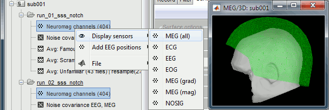
For each subject, all the runs have been registered to a common head position with MaxFilter. To verify this, select all the channel files within one subject, right-click > Display sensors > MEG (all). The surfaces representing the MEG helmet are perfectly overlapping for all the runs. When the runs are not aligned, it looks like this.

This means that we can safely average or compare the MEG sensor values across runs within one subject. However, it is not reliable to average MEG recordings across subjects, because of the anatomical differences between subjects.

This doesn't mean that we can estimate the sources only once per subject. We have computed different SSP projectors and different bad channels for the each acquisition run. To be able to use this information efficiently we should estimate the sources for the trial averages for each run separately, then average the sources across runs.

The forward model is the same for all the runs within one subject, therefore it can be computed for the first run and copied to all the other runs.

Objectives [TODO]

The objectives for this tutorial are to reproduce the analysis presented in the following documents:

Wakeman DG, Henson RN, A multi-subject, multi-modal human neuroimaging dataset
Scientific Data (2015)
Wakeman DG, Henson RN, Functional and structural connctivity in face processing: MEG, EEG, fMRI, MRI and DWI data, Biomag 2016
SPM12 manual, chapter 41: Multimodal, Multisubject data fusion

Summary of the results we will compute in this tutorial:

Subject and grand averages for each condition (Famous, Unfamiliar, Scrambled).
Normalization of these averages (Z-score for the sources, or ERS/D for the time-frequency maps).
Contrast between faces (Famous+Unfamiliar) and non-faces (Scrambled).
Contrast between famous faces and unfamiliar faces.
Two constrast measures: first a difference of grand averages, then a t-test across subjects.
Sensors of interest: EEG070 (or EEG060 or EEG065 if EEG070 is marked as bad)

Expected effects:

OFA: Bilateral occipital face area
FFA: Bilateral fusiform face area
STS: Right superior temporal sulcus
Around 170ms (N170): Difference between Faces and Scrambled.
After 250ms: Difference between Famous and Unfamiliar.

The methodology that we will follow for computing the averages and the other statistics are described in the tutorial "Workflows".

Subject averages: Famous, Unfamiliar, Scrambled

We will start by computing the subject-level averages for all the data types we have: sensor-level recordings, source maps and time-frequency results. We will use a weighted average to group the results we have for each run (weighted by the number of good trials). We want to compute the averages for each experimental condition separately (famous, unfamiliar, scrambled).

Since the files are already selected in the interface, we will also compute a grand average across subject. In this context, we will consider that each subject has the same weight in the gran average (option "weighted" not selected). Note that it is not accurate to average MEG recordings across subjects, but we can do it just to get a general idea (more information).

MEG/EEG

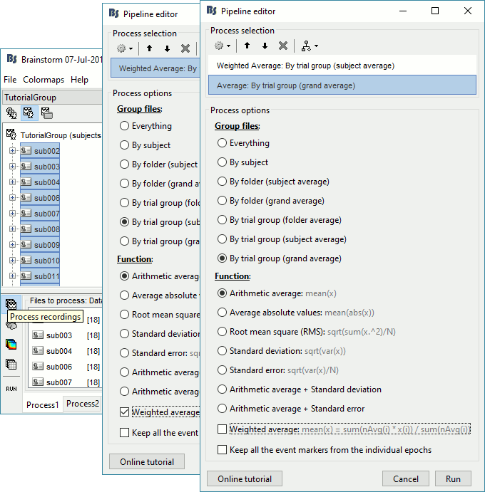
Drag and drop all the subjects in Process1. Select button [Process recordings].
Select process Average > Average files: By trial group (subject average)
Arithmetic average, Weighted
Add process Average > Average files: By trial group (grand average)
Arithmetic average, Not weighted
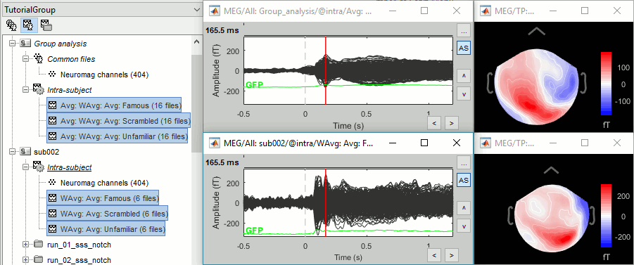
In output, you get three grand averages in the "Group analysis/Inter-subject" folder (top), and three subject averages per subject in the "intra-subject" folders (bottom).

Sources

Keep all the subjects selected in Process1. Select button [Process sources].
If you run the averaging process directly with this file selection, it would average together the MEG and the EEG sources (36 files selected per subject instead of 18). To average separately the two modalities, we can use the Filter box at the bottom-right corner of the Brainstorm window. Enter "EEG" and it would select only the files with a comment including the tag "EEG".
Select process Average > Average files: By trial group (subject average)
EEG source files only, Arithmetic average, Weighted
Add process File > Set tag: EEG.
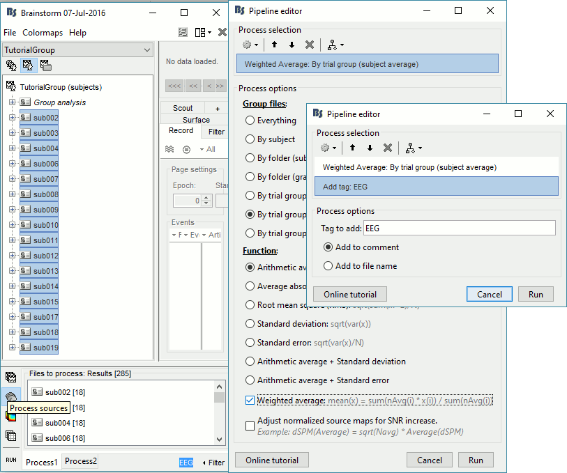
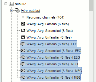
Repeat the same steps with the MEG source files (select all subjects, filter, average, tag).
This time, we cannot compute a grand average directly because the source spaces used to estimate the brain activity do not match between subjects. We will have to go through an additional step of projection on a template anatomy. We will also wait to have normalized the source maps before displaying them.

Time-frequency

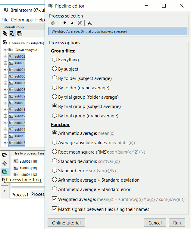
Keep all the subjects selected in Process1. Select button [Process time-freq].
Make sure you reset the Filter search box at the bottom-right of the Brainstorm window.
Run process Average > Average files: By trial group (subject average)
Arithmetic average, Weighted, Match signals
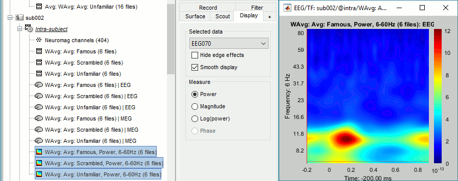
Like for the sources, we will first normalize the tim-frequency maps with respect with a baseline before computing grandoup averages.
We can average the time-frequency files across runs (it is as valid as averaging the MEG or EEG signals across subjects). But we need to select this option "match signals between files using their names" to account for the variable number of bad channels we may have across runs or subjects.

Subject averages: Faces

One of the constrast we want to study is faces (Famous and Unfamiliar) vs non-faces (Scrambled). We need to re-average the Famous and Unfamiliar averages together.

MEG/EEG

In Process2: FilesA = all the Famous subject averages, FilesB = all the Unfamiliar subject averages. The subjects must be in the same order in the two lists because the process will process the files by pairs of files (A,B).
Select process Other > Average A&B: Weighted.
Add process File > Set comment: Comment = "WAvg: Avg: Faces"
Add process Average > Average files: By trial group (subject average): Not weighted
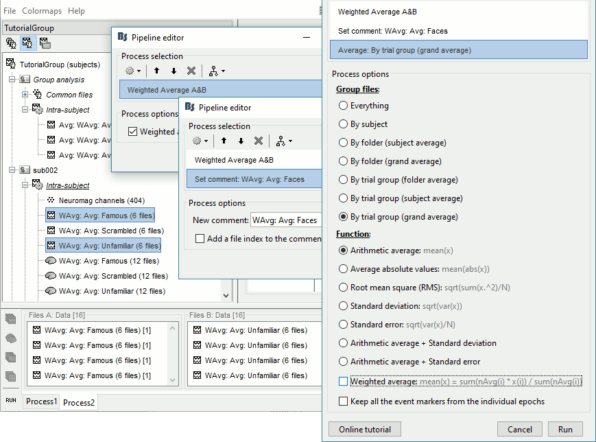
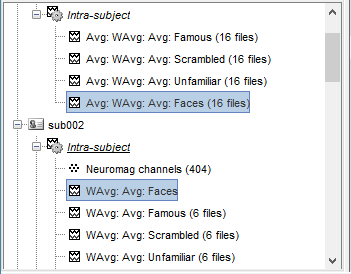
Selecting that many files from the database explorer can be long when done manually, but can be done very efficiently from a script. Check out the script equivalent at the end of this page.
It creates one new average for each pair (A,B) and compute the grand average for condition Faces.

Sources

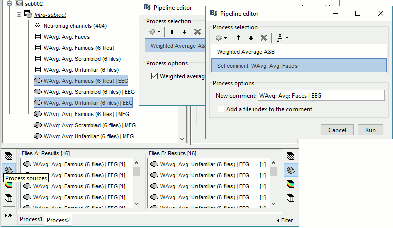
In Process2: FilesA = all the Famous subject averages (EEG only) [Process sources]
In Process2: FilesB = all the Unfamiliar subject averages (EEG only) [Process sources]
Make sure the order of the files matches in the two lists.
Select process Other > Average A&B: Weighted.
Add process File > Set comment: Comment = "WAvg: Avg: Faces | EEG"
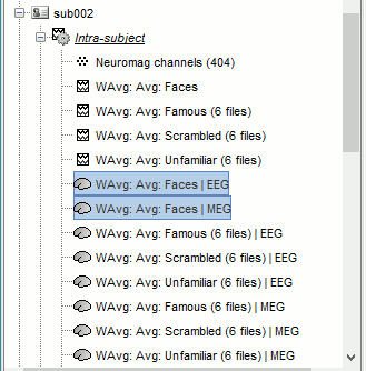
Repeat the same steps for the MEG sources.

Time-frequency

In Process2: FilesA = all the Famous subject averages (EEG only) [Process timefreq]
In Process2: FilesB = all the Unfamiliar subject averages (EEG only) [Process timefreq]
Select process Other > Average A&B: Weighted.
Add process File > Set comment: Comment = "WAvg: Avg: Faces"
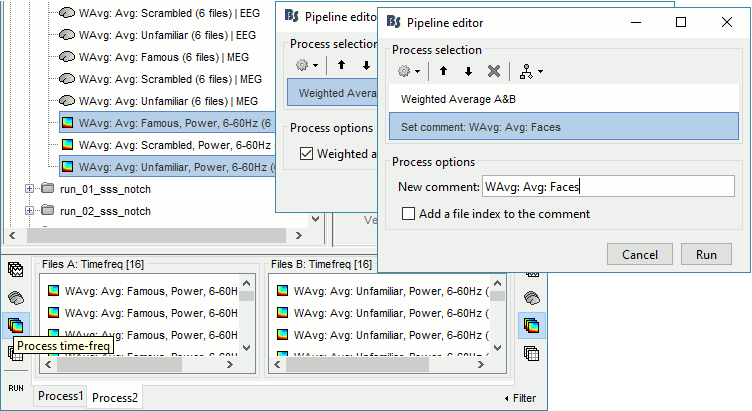
In output: the average for the Face condition, for each subject.

Subject averages: Within-subject differences

To detect correctly the differences between two conditions at the source level, we need to estimate the differences of the conditions for each subject before normalizing them (see tutorial Worflows).

Sources: Faces - Scrambled

In Process2: FilesA = all the Faces subject averages (EEG only) [Process sources]
In Process2: FilesB = all the Scrambled subject averages (EEG only) [Process sources]
Select process Difference > Difference A-B: Do not use absolute values.
Add process File > Set comment: Comment=Faces - Scrambled | EEG
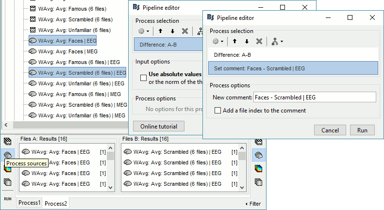
Repeat the same steps for the MEG sources.

Sources: Famous - Unfamiliar

In Process2: FilesA = all the Famous subject averages (EEG only) [Process sources]
In Process2: FilesB = all the Unfamiliar subject averages (EEG only) [Process sources]
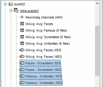
Select process Difference > Difference A-B: Do not use absolute values.
Add process File > Set comment: Comment=Famous - Unfamiliar | EEG
Repeat the same steps for the MEG sources.

Subject averages: Filter and normalize

Before comparing the averages across subjects we are going to low-pass filter the signals below 32Hz (to smooth possible latency differences between subjects) and normalize the source and time-frequency values with respect with a baseline (see tutorial Worflows).

MEG/EEG

In Process1, select all the Intra-subject folders from all the subjects, select [Process recordings]. For a faster selection, you can use the view "Functional data (sorted by conditions)".
Select process Pre-process > Band-pass filter: 0Hz-32Hz, MEG,EEG, Mirror, Overwrite
Add process Extract > Extract time: Time window=[-200,900]ms
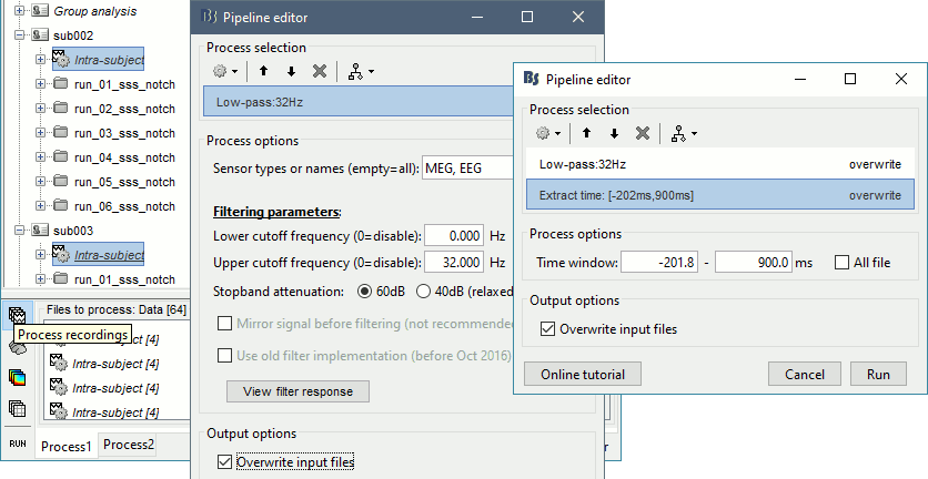
Two tags are added at the end of the comments of the averaged recordings.

Sources

In Process1, select all the Intra-subject folders from all the subjects, select [Process sources].
Select process Pre-process > Band-pass filter: 0Hz-32Hz, MEG,EEG, Mirror, Overwrite
Add process Extract > Extract time: Time window=[-200,900]ms
Add process Standardize > Baseline normalization: Baseline=[-200,-5]ms, Z-score, Overwrite
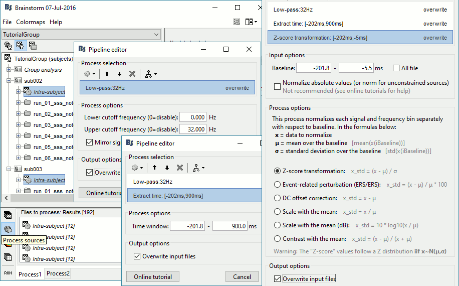
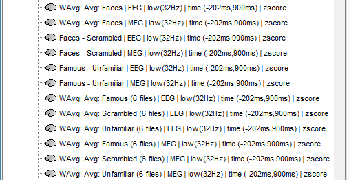
Three tags are added at the end of the comments of the averaged sources.

Time-frequency

In Process1, select all the Intra-subject folders from all the subjects, select [Process time-freq].
Run process Standardize > Baseline normalization: Baseline=[-200,-5]ms, ERS/ERD, Overwrite
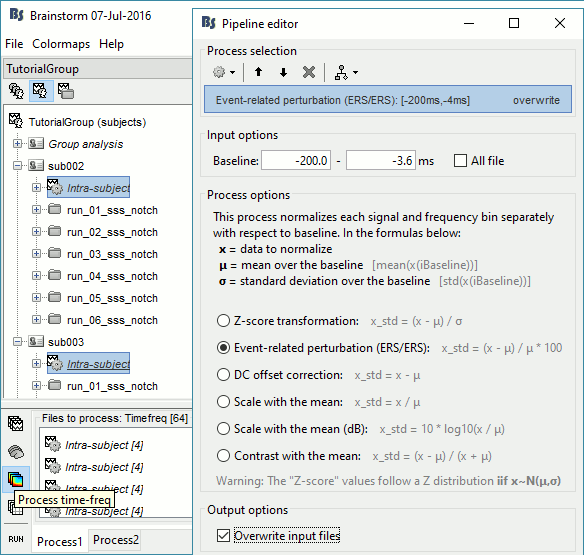
One tag is added at the end of the comments of the averaged time-frequency maps.

Subject averages: Screen captures

Now we have all the measures ready to be compared across subjects: MEG/EEG, sources, time-frequency. Let's take a few screen captures to make sure the primary visual response look good for all the subjects. The screen captures below represent from left to right:

Faces: EEG recordings
Faces: MEG sources at 107ms
Faces: Time-frequency for EEG070

sub002

sub003

sub004

sub006

sub007

sub008

sub009

sub010

sub011

sub012

sub013

sub014

sub015

sub017

sub018

sub019

Group analysis: MEG/EEG

Grand averages

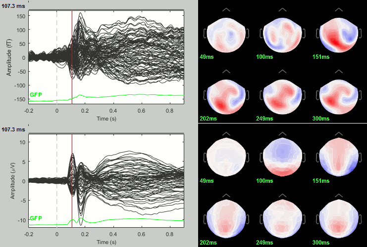
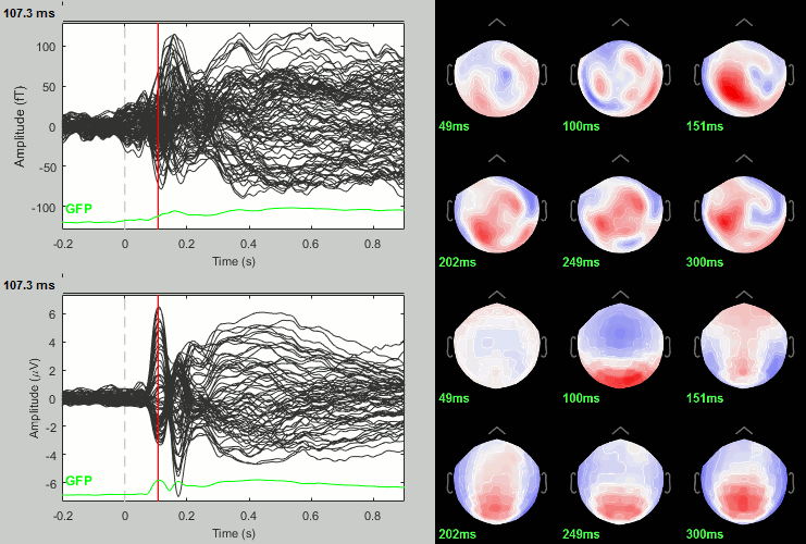
We have already computed the group averages for all the conditions. We will not look to much at these results, as we are more interested at the contrasts between conditions. Here are screen captures for all the averages (top=MEG, bottom=EEG). Topography at [50,100,150,200,250,300]ms.

Faces: Famous / Unfamiliar

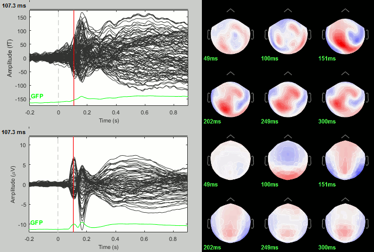
Scrambled

Faces - Scrambled: Differences of averages

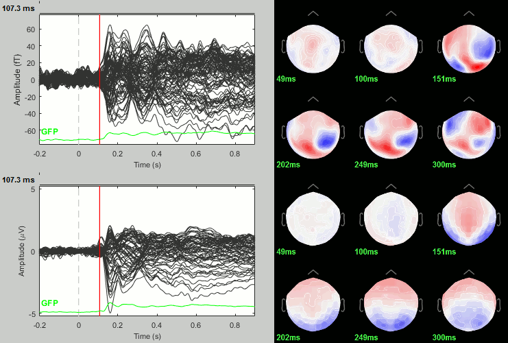
We could compute the contrasts directly from the grand averages, but we will do it from the subject averages because it will be the same file selection as for the statistics.

In Process2: FilesA = all the Faces subject averages (from the Intra-subject folders).
In Process2: FilesB = all the Scrambled subject averages (from the Intra-subject folders).
Run process: Test > Difference of means: Arithmetic average, Not weighted.
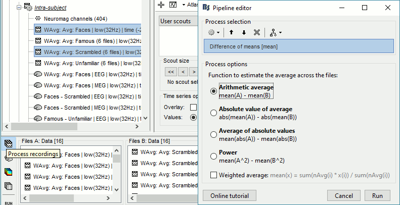
Rename the file: Faces - Scrambled (top=MEG, bottom=EEG).

Faces - Scrambled: Student t-test

In Process2: Keep the same file selection.
Run process: Test > Parametric test: Paired: All file, All sensors, No average, two-tailed.
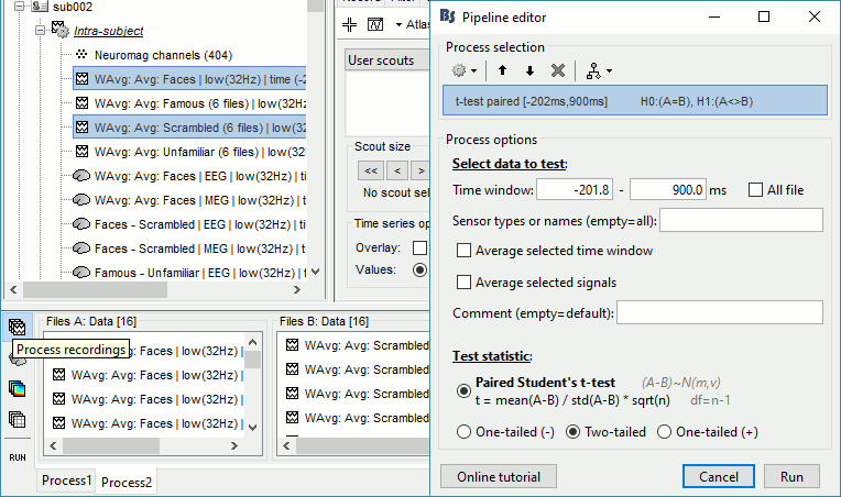
Rename the file: Faces - Scrambled: Parametric t-test. Display with p<0.05, FDR-corrected.
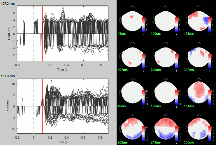
You can run other tests in a similar way, with almost identical results.
Process: Test > Permutation test: Paired: All file, All sensors, Paired t-test, 1000 randomizations.
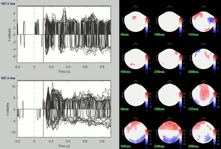
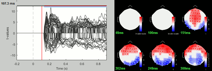
Process: Test > FieldTrip: ft_timelockstatistics: All file, EEG, Paired t-test, 1000 randomizations, correction=cluster, cluster alpha=0.05. The cluster-based statistics must be executed on one type of sensors at a time (EEG, MEG MAG, MEG GRAD), because it tries to identify spatio-temporal clusters which groups adjacent sensors.

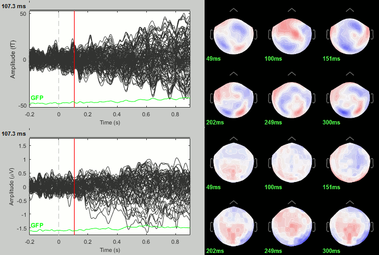
Famous - Unfamiliar: Differences of averages

In Process2: FilesA = all the Famous subject averages (from the Intra-subject folders).
In Process2: FilesB = all the Unfamiliar subject averages (from the Intra-subject folders).
Run process: Test > Difference of means: Arithmetic average, Not weighted.
Rename the file: Famous - Unfamiliar.

Famous - Unfamiliar: Student t-test

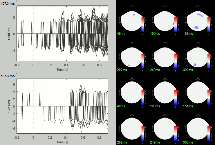
In Process2: Keep the same file selection.
Run process: Test > Parametric test: Paired: All file, All sensors, No average, two-tailed.
Rename the file: Faces - Scrambled: Parametric t-test. Display with p<0.05, FDR-corrected.

Group analysis: Sources

Projet sources on template

The sources were estimated on the individual anatomy of each subject, the resulting cortical source maps cannot be averaged directly. We need first to re-interpolate all the individual results on a common template (the ICBM152 brain, available in the "default anatomy" folder of the protocol). We also need to extract the absolute values for these source maps: the sign of the minimum norm maps are relative to the orientation of the current with respect to the surface normal, which can vary between subjects.

In Process1, select all the Intra-subject folders from all the subjects, select [Process recordings]. For a faster selection, you can use the view "Functional data (sorted by conditions)".
Select process Pre-process > Absolute values: Sensor types=MEG,EEG, Overwrite.
Add process Sources > Project on default anatomy.
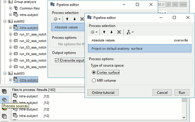
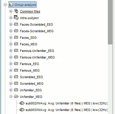
All the 192 subject averages are projected in the same folder "Group analysis / Intra-subject". Re-organize all the projected source files in new folders, one folder per condition.
To create a folder, right-click on Group analysis > New folder. To move a file to the new folder: drag and drop it in the database explorer or use the keyboard shortcuts Ctrl+X/Ctrl+V.

Faces - Scrambled: Differences of averages (MEG)

In Process2: FilesA = all the source files in Group_analysis/Faces_MEG.
In Process2: FilesB = all the source files in Group_analysis/Scrambled_MEG.
Run process Test > Difference of means: Arithmetic average, Not weighted.
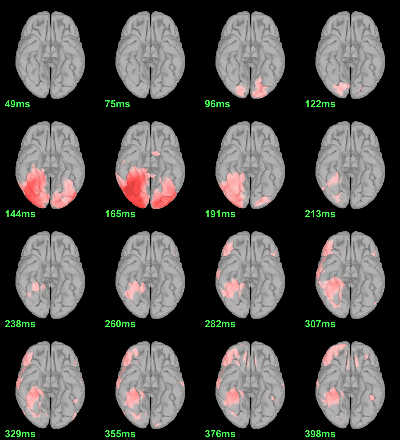
Regions of interest: OFA (Occipital Face Area), FFA (Fusiform Face Area), V1.

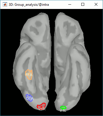
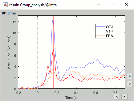
Faces - Scrambled: Parametric Student t-test (MEG)

In Process2: FilesA = all the source files in Group_analysis/Faces_MEG.
In Process2: FilesB = all the source files in Group_analysis/Scrambled_MEG.
Run process Test > Parametric test: Paired: All file, No average, two-tailed.
Screen capture: p<0.05 FDR-corrected
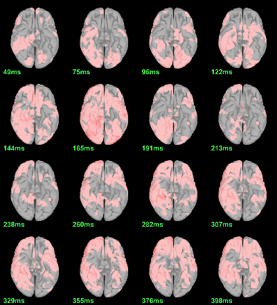
This test the hypothesis H0:[mean(abs(Faces))=mean(abs(Scrambled))].
This measure is not appropriate to properly identify the differences between the two conditions because it is insensitive to the sign of the sources within each subject.

Faces - Scrambled: Parametric Chi2 test (MEG) [TODO]

In Process1, select all the source files in Group_analysis/Faces-Scrambled_MEG.
Run process Test > Parametric test against zero: All file, One-sample Chi2-test two-tailed.
Screen capture: p<0.05 FDR-corrected
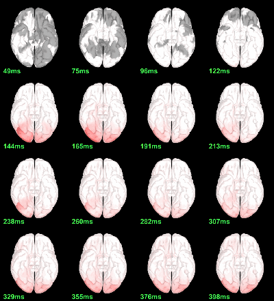
This tests the hypotesis H0:[mean_subject(|Faces-Scrambled|) = 0]
This test is appropriate to detect the differences between the two conditions, but cannot determine which condition is stronger.
ERROR: There is something wrong here, because everything is significant even with a Bonferroni correction for multiple comparisons. Either the test is not adapted, or it's not coded properly.

Faces - Scrambled (EEG) [TODO]

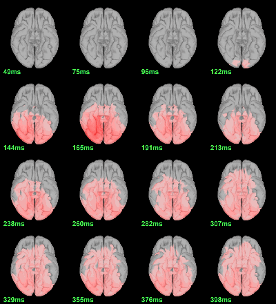
Repeat the same operations with the EEG sources.
Difference of averages:
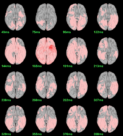
Parametric Student t-test: [mean(abs(Faces))=mean(abs(Scrambled))], p<0.05 FDR-corrected
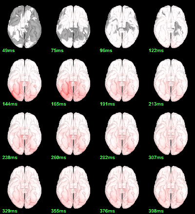
Paramtric Chi2 t-test: [mean_subject(|Faces-Scrambled|) = 0], p<0.05 FDR-corrected

Scripting

The following script from the Brainstorm distribution reproduces the analysis presented in this tutorial page: brainstorm3/toolbox/script/tutorial_visual_group.m

function tutorial_visual_group(ProtocolName, reports_dir)
% TUTORIAL_VISUAL_GROUP: Runs the Brainstorm/SPM group analysis pipeline (group analysis, BIDS VERSION)
%
% ONLINE TUTORIALS: 
%    - https://neuroimage.usc.edu/brainstorm/Tutorials/VisualSingle
%    - https://neuroimage.usc.edu/brainstorm/Tutorials/VisualGroup
%
% INPUTS:
%    - ProtocolName : Name of the protocol in which the recordings for the 19 subjects have been imported (TutorialVisual or TutorialGroup)
%                     This folder must include: the run-level averages (recordings and time-frequency) and the source kernels for each run
%    - reports_dir  : If defined, exports all the reports as HTML to this folder

% @=============================================================================
% This function is part of the Brainstorm software:
% https://neuroimage.usc.edu/brainstorm
% 
% Copyright (c) University of Southern California & McGill University
% This software is distributed under the terms of the GNU General Public License
% as published by the Free Software Foundation. Further details on the GPLv3
% license can be found at http://www.gnu.org/copyleft/gpl.html.
% 
% FOR RESEARCH PURPOSES ONLY. THE SOFTWARE IS PROVIDED "AS IS," AND THE
% UNIVERSITY OF SOUTHERN CALIFORNIA AND ITS COLLABORATORS DO NOT MAKE ANY
% WARRANTY, EXPRESS OR IMPLIED, INCLUDING BUT NOT LIMITED TO WARRANTIES OF
% MERCHANTABILITY AND FITNESS FOR A PARTICULAR PURPOSE, NOR DO THEY ASSUME ANY
% LIABILITY OR RESPONSIBILITY FOR THE USE OF THIS SOFTWARE.
%
% For more information type "brainstorm license" at command prompt.
% =============================================================================@
%
% Author: Francois Tadel, Elizabeth Bock, 2016-2018

% ===== CHECK PROTOCOL =====
% Start Brainstorm without the GUI
if ~brainstorm('status')
    brainstorm nogui
end
% Output folder for reports
if (nargin < 2) || isempty(reports_dir) || ~isdir(reports_dir)
    reports_dir = [];
end
% You have to specify the folder in which the tutorial dataset is unzipped
if (nargin < 1) || isempty(ProtocolName)
    ProtocolName = 'TutorialGroup';
end
% Select current protocol
iProtocol = bst_get('Protocol', ProtocolName);
if isempty(iProtocol)
    error(['Unknown protocol: ' ProtocolName]);
end
if (iProtocol ~= bst_get('iProtocol'))
    gui_brainstorm('SetCurrentProtocol', iProtocol);
end
% Process: Select results files in: sub-01/sub-01_ses-meg_task-facerecognition_run-01_proc-sss_meg_notch
sFiles = bst_process('CallProcess', 'process_select_files_results', [], [], ...
    'subjectname', 'sub-01', ...
    'condition',   'sub-01_ses-meg_task-facerecognition_run-01_proc-sss_meg_notch');
if isempty(sFiles)
    error(['No source files available in folder: sub-01/sub-01_ses-meg_task-facerecognition_run-01_proc-sss_meg_notch.' 10 ...
           'You should run tutorial_visual_single first, or download the ' 10 ...
           'protocol TutorialGroup.zip from the Brainstorm website.']);
end
% Process: Select file comments with tag: Unconstr
sFiles = bst_process('CallProcess', 'process_select_tag', sFiles, [], 'tag', 'Unconstr');
if ~isempty(sFiles)
    isUnconstrained = 1;
else
    isUnconstrained = 0;
end
% Start a new report
bst_report('Start');


% ===== DELETE ALL THE EXISTING FILES =====
GroupSubjectName = bst_get('NormalizedSubjectName');
DirIntra = bst_get('DirAnalysisIntra');
% Delete group analysis
[sSubject, iSubject] = bst_get('Subject', GroupSubjectName);
if ~isempty(sSubject)
    db_delete_subjects(iSubject);
end
% Get all the files in the intra subjects
sAvgSrc = bst_process('CallProcess', 'process_select_files_data', [], [], ...
    'subjectname',   'All', ...
    'condition',     DirIntra, ...
    'includeintra',  1);
% If there are existing files: delete the contents of the folders
if ~isempty(sAvgSrc)
    % Get the base folder of the protocol
    ProtocolInfo = bst_get('ProtocolInfo', iProtocol);
    % Get all the folders
    AllIntraDir = unique(cellfun(@bst_fileparts, {sAvgSrc.FileName}, 'UniformOutput', 0));
    % Loop over the intra folders
    for iSubj = 1:length(AllIntraDir)
        % Get all the files
        subjIntraDir = dir(fullfile(ProtocolInfo.STUDIES, AllIntraDir{iSubj}, '*.mat'));
        subjIntraFiles = setdiff({subjIntraDir.name}, 'brainstormstudy.mat');
        % Delete all the files
        for iFile = 1:length(subjIntraFiles)
            delete(fullfile(ProtocolInfo.STUDIES, AllIntraDir{iSubj}, subjIntraFiles{iFile}));
        end
    end
    % Reload protocol
    db_reload_database(iProtocol);
end


%% ===== SUBJECT AVERAGES: FAMOUS, UNFAMILIAR, SCRAMBLED ==============================
%  ====================================================================================

% ===== SUBJECT AVERAGE: MEG+EEG =====
% Process: Select data files in: */*/Avg
sAvgRun = bst_process('CallProcess', 'process_select_files_data', [], [], ...
    'subjectname', 'All', ...
    'tag',         'Avg');
% Process: Weighted Average: By trial group (subject average)
sAvgSubj = bst_process('CallProcess', 'process_average', sAvgRun, [], ...
    'avgtype',    6, ...  % By trial group (subject average)
    'avg_func',   1, ...  % Arithmetic average:  mean(x)
    'weighted',   1, ...
    'keepevents', 1);
% Process: Average: By trial group (grand average)
sAvgGroup = bst_process('CallProcess', 'process_average', sAvgSubj, [], ...
    'avgtype',    7, ...  % By trial group (grand average)
    'avg_func',   1, ...  % Arithmetic average:  mean(x)
    'weighted',   0, ...
    'keepevents', 0);

% ===== SUBJECT AVERAGES: SOURCES (EEG) =====
% Process: Select source files in: */*/EEG
sAvgRunSrcEeg = bst_process('CallProcess', 'process_select_files_results', [], [], 'tag', 'EEG');
% Process: Weighted Average: By trial group (subject average) - EEG
sAvgSubjSrcEeg = bst_process('CallProcess', 'process_average', sAvgRunSrcEeg, [], ...
    'avgtype',         6, ...  % By trial group (subject average)
    'avg_func',        1, ...  % Arithmetic average:  mean(x)
    'weighted',        1, ...
    'scalenormalized', 0);
% Process: Add tag: EEG
sAvgSubjSrcEeg = bst_process('CallProcess', 'process_add_tag', sAvgSubjSrcEeg, [], ...
    'tag',    'EEG', ...
    'output', 1);  % Add to comment

% ===== SUBJECT AVERAGES: SOURCES (MEG) =====
% Process: Select source files in: */*/MEG
sAvgRunSrcMeg = bst_process('CallProcess', 'process_select_files_results', [], [], 'tag', 'MEG');
% Process: Weighted Average: By trial group (subject average) - MEG
sAvgSubjSrcMeg = bst_process('CallProcess', 'process_average', sAvgRunSrcMeg, [], ...
    'avgtype',         6, ...  % By trial group (subject average)
    'avg_func',        1, ...  % Arithmetic average:  mean(x)
    'weighted',        1, ...
    'scalenormalized', 1);
% Process: Add tag: MEG
sAvgSubjSrcMeg = bst_process('CallProcess', 'process_add_tag', sAvgSubjSrcMeg, [], ...
    'tag',    'MEG', ...
    'output', 1);  % Add to comment

% ===== SUBJECT AVERAGES: TIMEFREQ =====
% Process: Select time-frequency files in: */*
sAvgRunTf = bst_process('CallProcess', 'process_select_files_timefreq', [], []);
% Process: Weighted Average: By trial group (subject average)
sAvgSubjTf = bst_process('CallProcess', 'process_average', sAvgRunTf, [], ...
    'avgtype',         6, ...  % By trial group (subject average)
    'avg_func',        1, ...  % Arithmetic average:  mean(x)
    'weighted',        1, ...
    'scalenormalized', 1);



%% ===== SUBJECT AVERAGES: FACES ======================================================
%  ====================================================================================

% ===== FACES AVERAGE: MEG+EEG ======
% Process: Select data files in: */*
sAllData = bst_process('CallProcess', 'process_select_files_data', [], [], ...
    'subjectname',   'All', ...
    'includeintra',  1);
% Process: Select file comments with tag: "WAvg: Avg: Famous (6 files)"
sAvgSubjFamous = bst_process('CallProcess', 'process_select_tag', sAllData, [], 'tag', 'WAvg: Avg: Famous (6 files)');
% Process: Select file comments with tag: "WAvg: Avg: Unfamiliar (6 files)"
sAvgSubjUnfamiliar = bst_process('CallProcess', 'process_select_tag', sAllData, [],  'tag', 'WAvg: Avg: Unfamiliar (6 files)');
% Process: Weighted Average A&B
sAvgSubjFaces = bst_process('CallProcess', 'process_average_ab', sAvgSubjFamous, sAvgSubjUnfamiliar, ...
    'weighted', 1);
% Process: Add tag: Faces
sAvgSubjFaces = bst_process('CallProcess', 'process_add_tag', sAvgSubjFaces, [], ...
    'tag',    'Faces', ...
    'output', 2);  % Add to file name
% Process: Set comment
sAvgSubjFaces = bst_process('CallProcess', 'process_set_comment', sAvgSubjFaces, [], ...
    'tag',     'WAvg: Avg: Faces', ...
    'isindex', 0);
% Process: Average: By trial group (grand average)
sAvgGroupFaces = bst_process('CallProcess', 'process_average', sAvgSubjFaces, [], ...
    'avgtype',    7, ...  % By trial group (grand average)
    'avg_func',   1, ...  % Arithmetic average:  mean(x)
    'weighted',   0, ...
    'keepevents', 0);

% ===== FACES AVERAGE: SOURCES (EEG) ======
% Process: Select source files in: */*/EEG
sSrcEeg = bst_process('CallProcess', 'process_select_files_results', [], [], ...
    'subjectname',   'All', ...
    'tag',           'EEG', ...
    'includeintra',  1);
% Process: Select file comments with tag: "WAvg: Avg: Famous"
sAvgSubjFamousSrcEeg = bst_process('CallProcess', 'process_select_tag', sSrcEeg, [], 'tag', 'WAvg: Avg: Famous');
% Process: Select file comments with tag: "WAvg: Avg: Unfamiliar"
sAvgSubjUnfamiliarSrcEeg = bst_process('CallProcess', 'process_select_tag', sSrcEeg, [], 'tag', 'WAvg: Avg: Unfamiliar');
% Process: Weighted Average A&B
sAvgSubjFacesSrcEeg = bst_process('CallProcess', 'process_average_ab', sAvgSubjFamousSrcEeg, sAvgSubjUnfamiliarSrcEeg, ...
    'weighted',        1, ...
    'scalenormalized', 1);
% Process: Add tag: Faces
sAvgSubjFacesSrcEeg = bst_process('CallProcess', 'process_add_tag', sAvgSubjFacesSrcEeg, [], ...
    'tag',    'Faces', ...
    'output', 2);  % Add to file name
% Process: Set comment
sAvgSubjFacesSrcEeg = bst_process('CallProcess', 'process_set_comment', sAvgSubjFacesSrcEeg, [], ...
    'tag',     'WAvg: Avg: Faces | EEG', ...
    'isindex', 0);

% ===== FACES AVERAGE: SOURCES (MEG) ======
% Process: Select source files in: */*
sSrcMeg = bst_process('CallProcess', 'process_select_files_results', [], [], ...
    'subjectname',   'All', ...
    'tag',           'MEG', ...
    'includeintra',  1);
% Process: Select file comments with tag: Famous
sAvgSubjFamousSrcMeg = bst_process('CallProcess', 'process_select_tag', sSrcMeg, [], 'tag', 'Famous');
% Process: Select file comments with tag: Unfamiliar
sAvgSubjUnfamiliarSrcMeg = bst_process('CallProcess', 'process_select_tag', sSrcMeg, [], 'tag', 'Unfamiliar');
% Process: Weighted Average A&B
sAvgSubjFacesSrcMeg = bst_process('CallProcess', 'process_average_ab', sAvgSubjFamousSrcMeg, sAvgSubjUnfamiliarSrcMeg, ...
    'weighted',        1, ...
    'scalenormalized', 1);
% Process: Add tag: Faces
sAvgSubjFacesSrcMeg = bst_process('CallProcess', 'process_add_tag', sAvgSubjFacesSrcMeg, [], ...
    'tag',    'Faces', ...
    'output', 2);  % Add to file name
% Process: Set comment
sAvgSubjFacesSrcMeg = bst_process('CallProcess', 'process_set_comment', sAvgSubjFacesSrcMeg, [], ...
    'tag',     'WAvg: Avg: Faces | MEG', ...
    'isindex', 0);

% ===== FACES AVERAGE: TIMEFREQ ======
% Process: Select time-frequency files in: */*
sAllTf = bst_process('CallProcess', 'process_select_files_timefreq', [], [], ...
    'subjectname',   'All', ...
    'includeintra',  1);
% Process: Select file comments with tag: "WAvg: Avg: Famous"
sAvgSubjFamousTf = bst_process('CallProcess', 'process_select_tag', sAllTf, [], 'tag', 'WAvg: Avg: Famous');
% Process: Select file comments with tag: "WAvg: Avg: Unfamiliar"
sAvgSubjUnfamiliarTf = bst_process('CallProcess', 'process_select_tag', sAllTf, [], 'tag', 'WAvg: Avg: Unfamiliar');
% Process: Weighted Average A&B
sAvgSubjFacesTf = bst_process('CallProcess', 'process_average_ab', sAvgSubjFamousTf, sAvgSubjUnfamiliarTf, ...
    'weighted', 1);
% Process: Add tag: Faces
sAvgSubjFacesTf = bst_process('CallProcess', 'process_add_tag', sAvgSubjFacesTf, [], ...
    'tag',    'Faces', ...
    'output', 2);  % Add to file name
% Process: Set comment
sAvgSubjFacesTf = bst_process('CallProcess', 'process_set_comment', sAvgSubjFacesTf, [], ...
    'tag',     'WAvg: Avg: Faces', ...
    'isindex', 0);



%% ===== SUBJECT AVERAGES: WITHIN-SUBJECT DIFFERENCES =================================
%  ====================================================================================

% ===== FACES - SCRAMBLED: SOURCES EEG =====
% Process: Select source files in: */*/EEG
sSrcEeg = bst_process('CallProcess', 'process_select_files_results', [], [], ...
    'subjectname',   'All', ...
    'tag',           'EEG', ...
    'includeintra',  1);
% Process: Select file comments with tag: "WAvg: Avg: Faces"
sAvgSubjFacesSrcEeg = bst_process('CallProcess', 'process_select_tag', sSrcEeg, [], 'tag', 'WAvg: Avg: Faces');
% Process: Select file comments with tag: "WAvg: Avg: Scrambled"
sAvgSubjScrambledSrcEeg = bst_process('CallProcess', 'process_select_tag', sSrcEeg, [], 'tag', 'WAvg: Avg: Scrambled');
% Process: Difference: A-B
sDiffFacesSubjSrcEeg = bst_process('CallProcess', 'process_diff_ab', sAvgSubjFacesSrcEeg, sAvgSubjScrambledSrcEeg, ...
    'source_abs', 0);
% Process: Set comment
sDiffFacesSubjSrcEeg = bst_process('CallProcess', 'process_set_comment', sDiffFacesSubjSrcEeg, [], ...
    'tag',     'Faces - Scrambled | EEG', ...
    'isindex', 0);

% ===== FACES - SCRAMBLED: SOURCES MEG =====
% Process: Select source files in: */*/MEG
sSrcMeg = bst_process('CallProcess', 'process_select_files_results', [], [], ...
    'subjectname',   'All', ...
    'tag',           'MEG', ...
    'includeintra',  1);
% Process: Select file comments with tag: "WAvg: Avg: Faces"
sAvgSubjFacesSrcMeg = bst_process('CallProcess', 'process_select_tag', sSrcMeg, [], 'tag', 'WAvg: Avg: Faces');
% Process: Select file comments with tag: "WAvg: Avg: Scrambled"
sAvgSubjScrambledSrcMeg = bst_process('CallProcess', 'process_select_tag', sSrcMeg, [], 'tag', 'WAvg: Avg: Scrambled');
% Process: Difference: A-B
sDiffFacesSubjSrcMeg = bst_process('CallProcess', 'process_diff_ab', sAvgSubjFacesSrcMeg, sAvgSubjScrambledSrcMeg, ...
    'source_abs', 0);
% Process: Set comment
sDiffFacesSubjSrcMeg = bst_process('CallProcess', 'process_set_comment', sDiffFacesSubjSrcMeg, [], ...
    'tag',     'Faces - Scrambled | MEG', ...
    'isindex', 0);

% ===== FAMOUS - UNFAMILIAR: SOURCE EEG =====
% Process: Select file comments with tag: "WAvg: Avg: Famous"
sAvgSubjFamousSrcEeg = bst_process('CallProcess', 'process_select_tag', sSrcEeg, [], 'tag', 'WAvg: Avg: Famous');
% Process: Select file comments with tag: "WAvg: Avg: Unfamiliar"
sAvgSubjUnfamiliarSrcEeg = bst_process('CallProcess', 'process_select_tag', sSrcEeg, [], 'tag', 'WAvg: Avg: Unfamiliar');
% Process: Difference: A-B
sDiffFamousSubjSrcEeg = bst_process('CallProcess', 'process_diff_ab', sAvgSubjFamousSrcEeg, sAvgSubjUnfamiliarSrcEeg, ...
    'source_abs', 0);
% Process: Set comment
sDiffFamousSubjSrcEeg = bst_process('CallProcess', 'process_set_comment', sDiffFamousSubjSrcEeg, [], ...
    'tag',     'Famous - Unfamiliar | EEG', ...
    'isindex', 0);

% ===== FAMOUS - UNFAMILIAR: SOURCE MEG =====
% Process: Select file comments with tag: "WAvg: Avg: Famous"
sAvgSubjFamousSrcMeg = bst_process('CallProcess', 'process_select_tag', sSrcMeg, [], 'tag', 'WAvg: Avg: Famous');
% Process: Select file comments with tag: "WAvg: Avg: Unfamiliar"
sAvgSubjUnfamiliarSrcMeg = bst_process('CallProcess', 'process_select_tag', sSrcMeg, [], 'tag', 'WAvg: Avg: Unfamiliar');
% Process: Difference: A-B
sDiffFamousSubjSrcMeg = bst_process('CallProcess', 'process_diff_ab', sAvgSubjFamousSrcMeg, sAvgSubjUnfamiliarSrcMeg, ...
    'source_abs', 0);
% Process: Set comment
sDiffFamousSubjSrcMeg = bst_process('CallProcess', 'process_set_comment', sDiffFamousSubjSrcMeg, [], ...
    'tag',     'Famous - Unfamiliar | MEG', ...
    'isindex', 0);



%% ===== SUBJECT AVERAGES: FILTER AND NORMALIZE =======================================
%  ====================================================================================

% ===== FILTER: MEG+EEG =====
% Process: Select data files in: */Intra
sAvgData = bst_process('CallProcess', 'process_select_files_data', [], [], ...
    'subjectname',   'All', ...
    'condition',     DirIntra, ...
    'includeintra',  1);
% Process: Low-pass:32Hz
sAvgData = bst_process('CallProcess', 'process_bandpass', sAvgData, [], ...
    'sensortypes', 'MEG, EEG', ...
    'highpass',    0, ...
    'lowpass',     32, ...
    'attenuation', 'strict', ...  % 60dB
    'mirror',      0, ...
    'overwrite',   1);
% Process: Extract time: [-202ms,900ms]
sAvgData = bst_process('CallProcess', 'process_extract_time', sAvgData, [], ...
    'timewindow', [-0.2018, 0.9], ...
    'overwrite',  1);

% ===== FILTER AND NORMALIZE: SOURCES =====
% Process: Select source files in: */Intra
sAvgSrc = bst_process('CallProcess', 'process_select_files_results', [], [], ...
    'subjectname',   'All', ...
    'condition',     DirIntra, ...
    'includeintra',  1);
% Process: Low-pass:32Hz
sAvgSrc = bst_process('CallProcess', 'process_bandpass', sAvgSrc, [], ...
    'highpass',    0, ...
    'lowpass',     32, ...
    'attenuation', 'strict', ...  % 60dB
    'mirror',      0, ...
    'overwrite',   1);
% Process: Extract time: [-202ms,900ms]
sAvgSrc = bst_process('CallProcess', 'process_extract_time', sAvgSrc, [], ...
    'timewindow', [-0.2018, 0.9], ...
    'overwrite',  1);
% Process: Z-score transformation: [-202ms,-5ms]
sAvgSrc = bst_process('CallProcess', 'process_baseline_norm', sAvgSrc, [], ...
    'baseline',   [-0.2018, -0.005], ...
    'source_abs', 0, ...
    'method',     'zscore', ...  % Z-score transformation:    x_std = (x - μ) / σ
    'overwrite',  1);

% ===== NORMALIZE: TIMEFREQ =====
% Process: Select time-frequency files in: */Intra
sAvgTf = bst_process('CallProcess', 'process_select_files_timefreq', [], [], ...
    'subjectname',   'All', ...
    'condition',     DirIntra, ...
    'includeintra',  1);
% Process: Event-related perturbation (ERS/ERD): [-200ms,-4ms]
sAvgTf = bst_process('CallProcess', 'process_baseline_norm', sAvgTf, [], ...
    'baseline',  [-0.2, -0.004], ...
    'method',    'ersd', ...  % Event-related perturbation (ERS/ERD):    x_std = (x - μ) / μ * 100
    'overwrite', 1);

% Save report
ReportFile = bst_report('Save', []);
if ~isempty(reports_dir) && ~isempty(ReportFile)
    bst_report('Export', ReportFile, bst_fullfile(reports_dir, ['report_' ProtocolName '_1prepare.html']));
end



%% ===== SUBJECT AVERAGES: SCREEN CAPTURES ============================================
%  ====================================================================================
% Start a new report
bst_report('Start');
% Set colormap: local color scale
bst_colormaps('SetMaxMode', 'stat2', 'local');

% ===== FACES: RECORDINGS ======
% Process: Select data files in: */*/WAvg: Avg: Faces |
sAvgFaces = bst_process('CallProcess', 'process_select_files_data', [], [], ...
    'subjectname',   'All', ...
    'tag',           'WAvg: Avg: Faces |', ...
    'includeintra',  1);
% Process: Snapshot: Recordings time series
bst_process('CallProcess', 'process_snapshot', sAvgFaces, [], ...
    'target',         1, ...  % Sensor/MRI registration
    'modality',       1);     % MEG
% Process: Snapshot: Recordings time series
bst_process('CallProcess', 'process_snapshot', sAvgFaces, [], ...
    'target',         5, ...  % Recordings time series
    'modality',       4, ...  % EEG
    'time',           0.1055);

% ===== FACES: SOURCES MEG ======
% Process: Select source files in: */*/WAvg: Avg: Faces | MEG
sAvgFacesSrcMeg = bst_process('CallProcess', 'process_select_files_results', [], [], ...
    'subjectname',   'All', ...
    'condition',     DirIntra, ...
    'tag',           'WAvg: Avg: Faces | MEG', ...
    'includeintra',  1);
% Process: Snapshot: Sources (one time)
bst_process('CallProcess', 'process_snapshot', sAvgFacesSrcMeg, [], ...
    'target',         8, ...  % Sources (one time)
    'orient',         6, ...  % back
    'time',           0.1055, ...
    'threshold',      10);

% ===== FACES: TIME-FREQ EEG ======
% Process: Select time-frequency files in: */*/WAvg: Avg: Faces
sAvgFacesTf = bst_process('CallProcess', 'process_select_files_timefreq', [], [], ...
    'subjectname',   'All', ...
    'tag',           'WAvg: Avg: Faces', ...
    'includeintra',  1);
% Process: Snapshot: Time-frequency maps
bst_process('CallProcess', 'process_snapshot', sAvgFacesTf, [], ...
    'target',         14, ...  % Time-frequency maps
    'time',           0.1055, ...
    'rowname',        'EEG070');

% Save report
ReportFile = bst_report('Save', []);
if ~isempty(reports_dir) && ~isempty(ReportFile)
    bst_report('Export', ReportFile, bst_fullfile(reports_dir, ['report_' ProtocolName '_2snapshots.html']));
end



%% ===== GROUP ANALYSIS: FACES-SCRAMBLED: MEG/EEG =====================================
%  ====================================================================================
% Start a new report
bst_report('Start');
% Set colormap: global color scale
bst_colormaps('SetMaxMode', 'meg', 'global');
bst_colormaps('SetMaxMode', 'eeg', 'global');
% Set display properties for statistics: p<0.05, FDR-corrected
StatThreshOptions = bst_get('StatThreshOptions');
StatThreshOptions.pThreshold = 0.05;
StatThreshOptions.Correction = 'fdr';
StatThreshOptions.Control    = [1 2 3];
bst_set('StatThreshOptions', StatThreshOptions);

% ===== GRAND AVERAGES =====
% Process: Select data files in: Group_analysis/Intra
sAvgData = bst_process('CallProcess', 'process_select_files_data', [], [], ...
    'subjectname',   GroupSubjectName, ...
    'condition',     DirIntra, ...
    'includeintra',  1);
% Take screen captures
DataScreenCapture(sAvgData(1), 1, 1, '');
DataScreenCapture(sAvgData(2), 1, 1, '');
DataScreenCapture(sAvgData(3), 1, 1, '');
DataScreenCapture(sAvgData(4), 1, 1, '');
% Define function for screen captures
function DataScreenCapture(sFiles, isMEG, isEEG, Comment)
    if isMEG
        % Process: Snapshot: Recordings time series
        bst_process('CallProcess', 'process_snapshot', sFiles, [], ...
            'target',         5, ...  % Recordings time series
            'modality',       3, ...  % MEG (Magnetometers)
            'time',           0.1055, ...
            'Comment',        ['MEG MAG: ' Comment]);
        % Process: Snapshot: Recordings topography (contact sheet)
        bst_process('CallProcess', 'process_snapshot', sFiles, [], ...
            'target',         7, ...  % Recordings topography (contact sheet)
            'modality',       3, ...  % MEG (Magnetometers)
            'contact_time',   [0.050, 0.300], ...
            'contact_nimage', 6, ...
            'Comment',        ['MEG MAG: ' Comment]);
    end
    if isEEG
        % Process: Snapshot: Recordings time series
        bst_process('CallProcess', 'process_snapshot', sFiles, [], ...
            'target',         5, ...  % Recordings time series
            'modality',       4, ...  % EEG
            'time',           0.1055, ...
            'Comment',        ['EEG: ' Comment]);
        % Process: Snapshot: Recordings topography (contact sheet)
        bst_process('CallProcess', 'process_snapshot', sFiles, [], ...
            'target',         7, ...  % Recordings topography (contact sheet)
            'modality',       4, ...  % EEG
            'contact_time',   [0.050, 0.300], ...
            'contact_nimage', 6, ...
            'Comment',        ['EEG: ' Comment]);
    end
end

% ===== FACES-SCRAMBLED: MEAN DIFF =====
% Process: Select data files in: */DirIntra/"Avg: Faces | "
sSubjAvgFacesData = bst_process('CallProcess', 'process_select_files_data', [], [], ...
    'subjectname',   'All', ...
    'condition',     DirIntra, ...
    'tag',           'Avg: Faces | ', ...
    'includeintra',  1);
% Process: Select data files in: */DirIntra/"WAvg: Avg: Scrambled (6 files)"
sSubjAvgScrambledData = bst_process('CallProcess', 'process_select_files_data', [], [], ...
    'subjectname',   'All', ...
    'condition',     DirIntra, ...
    'tag',           'WAvg: Avg: Scrambled (6 files)', ...
    'includeintra',  1);
% Process: Difference of means [mean]
sDiffFacesData = bst_process('CallProcess', 'process_diff_mean', sSubjAvgFacesData, sSubjAvgScrambledData, ...
    'avg_func', 1, ...  % Arithmetic average mean(A) - mean(B)
    'weighted', 0);
% Process: Set comment
sDiffFacesData = bst_process('CallProcess', 'process_set_comment', sDiffFacesData, [], ...
    'tag',     'Faces - Scrambled', ...
    'isindex', 0);
% Take screen captures
DataScreenCapture(sDiffFacesData, 1, 1, sDiffFacesData.Comment);

% ===== FACES-SCRAMBLED: PARAMETRIC T-TEST =====
% Process: Select data files in: */DirIntra/"Avg: Faces | "
sSubjAvgFacesData = bst_process('CallProcess', 'process_select_files_data', [], [], ...
    'subjectname',   'All', ...
    'condition',     DirIntra, ...
    'tag',           'Avg: Faces | ', ...
    'includeintra',  1);
% Process: Select data files in: */DirIntra/"WAvg: Avg: Scrambled (6 files)"
sSubjAvgScrambledData = bst_process('CallProcess', 'process_select_files_data', [], [], ...
    'subjectname',   'All', ...
    'condition',     DirIntra, ...
    'tag',           'WAvg: Avg: Scrambled (6 files)', ...
    'includeintra',  1);
% Process: t-test paired [ALL]          H0:(A=B), H1:(A<>B)
sStatParamFacesData = bst_process('CallProcess', 'process_test_parametric2p', sSubjAvgFacesData, sSubjAvgScrambledData, ...
    'timewindow',    [], ...
    'sensortypes',   '', ...
    'isabs',         0, ...
    'avgtime',       0, ...
    'avgrow',        0, ...
    'Comment',       '', ...
    'test_type',     'ttest_paired', ...  % Paired Student's t-test        (A-B)~N(m,v)t = mean(A-B) / std(A-B) * sqrt(n)      df=n-1
    'tail',          'two');  % Two-tailed
% Process: Set comment
sStatParamFacesData = bst_process('CallProcess', 'process_set_comment', sStatParamFacesData, [], ...
    'tag',     'Faces - Scrambled: Parametric t-test', ...
    'isindex', 0);
% Take screen captures
DataScreenCapture(sStatParamFacesData, 1, 1, sStatParamFacesData.Comment);

% ===== FACES-SCRAMBLED: NON-PARAMETRIC T-TEST =====
% Process: Perm t-test paired [All]          H0:(A=B), H1:(A<>B)
sStatPermFacesData = bst_process('CallProcess', 'process_test_permutation2p', sSubjAvgFacesData, sSubjAvgScrambledData, ...
    'timewindow',     [], ...
    'sensortypes',    '', ...
    'isabs',          0, ...
    'avgtime',        0, ...
    'avgrow',         0, ...
    'iszerobad',      0, ...
    'Comment',        '', ...
    'test_type',      'ttest_paired', ...  % Paired Student's t-test T = mean(A-B) / std(A-B) * sqrt(n)
    'randomizations', 1000, ...
    'tail',           'two');  % Two-tailed
% Process: Set comment
sStatPermFacesData = bst_process('CallProcess', 'process_set_comment', sStatPermFacesData, [], ...
    'tag',     'Faces - Scrambled: Permutation t-test', ...
    'isindex', 0);
% Take screen captures
DataScreenCapture(sStatPermFacesData, 1, 1, sStatPermFacesData.Comment);

% ===== FACES-SCRAMBLED: CLUSTER T-TEST =====
% Process: FT t-test paired cluster [all EEG]          H0:(A=B), H1:(A<>B)
sStatClustFacesData = bst_process('CallProcess', 'process_ft_timelockstatistics', sSubjAvgFacesData, sSubjAvgScrambledData, ...
    'sensortypes',    'EEG', ...
    'timewindow',     [], ...
    'isabs',          0, ...
    'avgtime',        0, ...
    'avgchan',        0, ...
    'randomizations', 1000, ...
    'statistictype',  2, ...  % Paired t-test
    'tail',           'two', ...  % Two-tailed
    'correctiontype', 2, ...  % cluster
    'minnbchan',      0, ...
    'clusteralpha',   0.05);
% If FieldTrip is available and results were returned
if ~isempty(sStatClustFacesData)
    % Process: Set comment
    sStatClustFacesData = bst_process('CallProcess', 'process_set_comment', sStatClustFacesData, [], ...
        'tag',     'Faces - Scrambled: Cluster t-test EEG', ...
        'isindex', 0);
    % Take screen captures
    DataScreenCapture(sStatClustFacesData, 0, 1, sStatClustFacesData.Comment);
end


%% ===== GROUP ANALYSIS: FACES-SCRAMBLED: MEG/EEG =====================================
%  ====================================================================================
% ===== FAMOUS-UNFAMILIAR: MEAN DIFF =====
% Process: Select data files in: */DirIntra/"Avg: Famous | "
sSubjAvgFamousData = bst_process('CallProcess', 'process_select_files_data', [], [], ...
    'subjectname',   'All', ...
    'condition',     DirIntra, ...
    'tag',           'Avg: Famous (6 files)', ...
    'includeintra',  1);
% Process: Select data files in: */DirIntra/"WAvg: Avg: Unfamiliar (6 files)"
sSubjAvgUnfamiliarData = bst_process('CallProcess', 'process_select_files_data', [], [], ...
    'subjectname',   'All', ...
    'condition',     DirIntra, ...
    'tag',           'WAvg: Avg: Unfamiliar (6 files)', ...
    'includeintra',  1);
% Process: Difference of means [mean]
sDiffFamousData = bst_process('CallProcess', 'process_diff_mean', sSubjAvgFamousData, sSubjAvgUnfamiliarData, ...
    'avg_func', 1, ...  % Arithmetic average mean(A) - mean(B)
    'weighted', 0);
% Process: Set comment
sDiffFamousData = bst_process('CallProcess', 'process_set_comment', sDiffFamousData, [], ...
    'tag',     'Famous - Unfamiliar', ...
    'isindex', 0);
% Take screen captures
DataScreenCapture(sDiffFamousData, 1, 1, sDiffFamousData.Comment);

% ===== FAMOUS-UNFAMILIAR: PARAMETRIC T-TEST =====
% Process: t-test paired [All]          H0:(A=B), H1:(A<>B)
sStatParamFamousData = bst_process('CallProcess', 'process_test_parametric2p', sSubjAvgFamousData, sSubjAvgUnfamiliarData, ...
    'timewindow',    [], ...
    'sensortypes',   '', ...
    'isabs',         0, ...
    'avgtime',       0, ...
    'avgrow',        0, ...
    'Comment',       '', ...
    'test_type',     'ttest_paired', ...  % Paired Student's t-test        (A-B)~N(m,v)t = mean(A-B) / std(A-B) * sqrt(n)      df=n-1
    'tail',          'two');  % Two-tailed
% Process: Set comment
sStatParamFamousData = bst_process('CallProcess', 'process_set_comment', sStatParamFamousData, [], ...
    'tag',     'Famous - Unfamiliar: Parametric t-test', ...
    'isindex', 0);
% Take screen captures
DataScreenCapture(sStatParamFamousData, 1, 1, sStatParamFamousData.Comment);

% ===== FAMOUS-UNFAMILIAR: CLUSTER T-TEST =====
% Process: FT t-test paired cluster [all EEG]          H0:(A=B), H1:(A<>B)
sStatClustFamousData = bst_process('CallProcess', 'process_ft_timelockstatistics', sSubjAvgFamousData, sSubjAvgUnfamiliarData, ...
    'sensortypes',    'EEG', ...
    'timewindow',     [], ...
    'isabs',          0, ...
    'avgtime',        0, ...
    'avgchan',        0, ...
    'randomizations', 1000, ...
    'statistictype',  2, ...  % Paired t-test
    'tail',           'two', ...  % Two-tailed
    'correctiontype', 2, ...  % cluster
    'minnbchan',      0, ...
    'clusteralpha',   0.05);
% If FieldTrip is available and results were returned
if ~isempty(sStatClustFacesData)
    % Process: Set comment
    sStatClustFamousData = bst_process('CallProcess', 'process_set_comment', sStatClustFamousData, [], ...
        'tag',     'Famous - Unfamiliar: Cluster t-test EEG', ...
        'isindex', 0);
    % Take screen captures
    DataScreenCapture(sStatClustFamousData, 0, 1, sStatClustFamousData.Comment);
end

% Save report
ReportFile = bst_report('Save', []);
if ~isempty(reports_dir) && ~isempty(ReportFile)
    bst_report('Export', ReportFile, bst_fullfile(reports_dir, ['report_' ProtocolName '_3meeg.html']));
end



%% ===== FACES-SCRAMBLED: SOURCES (MEG) ===============================================
%  ====================================================================================
% Start a new report
bst_report('Start');

% ===== PROJECT SOURCES =====
% Process: Select source files in: */Intra
sAvgSrc = bst_process('CallProcess', 'process_select_files_results', [], [], ...
    'subjectname',   'All', ...
    'condition',     DirIntra, ...
    'includeintra',  1);
% Process: Absolute values / Norm for unconstrained
if isUnconstrained
    % Process: Unconstrained to flat map
    sAvgSrc = bst_process('CallProcess', 'process_source_flat', sAvgSrc, [], ...
        'method', 1);  % Norm: sqrt(x^2+y^2+z^2)
else
    sAvgSrc = bst_process('CallProcess', 'process_absolute', sAvgSrc, [], ...
        'overwrite', 1);
end
% Process: Project on default anatomy
sProjSrc = bst_process('CallProcess', 'process_project_sources', sAvgSrc, [], ...
    'headmodeltype', 'surface');  % Cortex surface
% Process: Spatial smoothing (3.00,abs)
sProjSrc = bst_process('CallProcess', 'process_ssmooth_surfstat', sProjSrc, [], ...
    'fwhm',       3, ...
    'overwrite',  1, ...
    'source_abs', 1);

% ===== MOVE FILES =====
% File tags / destination folder
ListTags = {'Avg: Faces | EEG',                 'Faces_EEG'; ...
            'Avg: Faces | MEG',                 'Faces_MEG'; ...
            'Avg: Famous (6 files) | EEG',      'Famous_EEG'; ...
            'Avg: Famous (6 files) | MEG',      'Famous_MEG'; ...
            'Avg: Unfamiliar (6 files) | EEG',  'Unfamiliar_EEG'; ...
            'Avg: Unfamiliar (6 files) | MEG',  'Unfamiliar_MEG'; ...
            'Avg: Scrambled (6 files) | EEG',   'Scrambled_EEG'; ...
            'Avg: Scrambled (6 files) | MEG',   'Scrambled_MEG'; ...
            'Faces - Scrambled | EEG',          'Faces-Scrambled_EEG'; ...
            'Faces - Scrambled | MEG',          'Faces-Scrambled_MEG'; ...
            'Famous - Unfamiliar | EEG',        'Famous-Unfamiliar_EEG'; ...
            'Famous - Unfamiliar | MEG',        'Famous-Unfamiliar_MEG'};
% Move group by group
for i = 1:size(ListTags,1)
    % Find names of files to move
    iTag = find(~cellfun(@(c)isempty(strfind(c, ListTags{i,1})), {sProjSrc.Comment}));
    if isempty(iTag)
        continue;
    end
    % Process: Move files
    bst_process('CallProcess', 'process_movefile', {sProjSrc(iTag).FileName}, [], ...
        'subjectname', GroupSubjectName, ...
        'folder',      ListTags{i,2});
end


% ===== LOOP ON MODALITY =====
AllModalities = {'MEG','EEG'};
for iMod = 1:length(AllModalities)
    % Selected modality for this loop
    Mod = AllModalities{iMod};
    
    % ===== |FACES-SCRAMBLED|: MEAN DIFF ======
    % Process: Select source files in: Group_analysis/Faces-Scrambled_MOD
    sDiffFaces = bst_process('CallProcess', 'process_select_files_results', [], [], ...
        'subjectname',   GroupSubjectName, ...
        'condition',     ['Faces-Scrambled_', Mod]);
    % Process: Weighted Average: By folder (grand average)
    sAbsDiffFaces = bst_process('CallProcess', 'process_average', sDiffFaces, [], ...
        'avgtype',         4, ...  % By folder (grand average)
        'avg_func',        1, ...  % Arithmetic average:  mean(x)
        'weighted',        0, ...
        'scalenormalized', 0);
    % Process: Set comment
    sAbsDiffFaces = bst_process('CallProcess', 'process_set_comment', sAbsDiffFaces, [], ...
        'tag',     ['mean(|Faces-Scrambled|) | ' Mod], ...
        'isindex', 0);
    % Process: Move files
    sAbsDiffFaces = bst_process('CallProcess', 'process_movefile', sAbsDiffFaces, [], ...
        'subjectname', GroupSubjectName, ...
        'folder',      DirIntra);
    % Colormap: Custom max: [-10,+10] Z
    bst_colormaps('SetMaxCustom', 'stat2', [], -10, 10);
    % Process: Snapshot: Sources (contact sheet)
    bst_process('CallProcess', 'process_snapshot', sAbsDiffFaces, [], ...
        'target',         9, ...  % Sources (contact sheet)
        'orient',         4, ...  % bottom
        'contact_time',   [0.05, 0.4], ...
        'contact_nimage', 16, ...
        'threshold',      30, ...
        'Comment',        [Mod ': mean(|Faces-Scrambled|)']);
    % Process: Snapshot: Sources (contact sheet)
    bst_process('CallProcess', 'process_snapshot', sAbsDiffFaces, [], ...
        'target',         9, ...  % Sources (contact sheet)
        'orient',         2, ...  % right
        'contact_time',   [0.05, 0.4], ...
        'contact_nimage', 16, ...
        'threshold',      30, ...
        'Comment',        [Mod ': mean(|Faces-Scrambled|)']);

    % ===== |FACES-SCRAMBLED|: PARAMETRIC CHI2-TEST ======
    % Process: Select source files in: Group_analysis/Faces-Scrambled_MOD
    sDiffFaces = bst_process('CallProcess', 'process_select_files_results', [], [], ...
        'subjectname',   GroupSubjectName, ...
        'condition',     ['Faces-Scrambled_' Mod]);
    % Process: Chi2-test [all]          H0:(|Zi| = 0)
    sChiParamFaces = bst_process('CallProcess', 'process_test_parametric1', sDiffFaces, [], ...
        'timewindow',    [], ...
        'scoutsel',      {}, ...
        'scoutfunc',     1, ...  % Mean
        'isnorm',        0, ...
        'avgtime',       0, ...
        'Comment',       '', ...
        'test_type',     'chi2_onesample', ...  % One-sample Chi2 test     Zi~N(0,1), i=1..nQ = sum(|Zi|^2)     Q~Chi2(n)
        'tail',          'two');  % Two-tailed
    % Process: Set comment
    sChiParamFaces = bst_process('CallProcess', 'process_set_comment', sChiParamFaces, [], ...
        'tag',     ['|Faces-Scrambled|=0: Parametric Chi2 test | ' Mod], ...
        'isindex', 0);
    % Process: Move files
    sChiParamFaces = bst_process('CallProcess', 'process_movefile', sChiParamFaces, [], ...
        'subjectname', GroupSubjectName, ...
        'folder',      DirIntra);
    % Set colormap: global color scale
    bst_colormaps('SetMaxMode', 'stat2', 'global');
    % Process: Snapshot: Sources (contact sheet)
    bst_process('CallProcess', 'process_snapshot', sChiParamFaces, [], ...
        'target',         9, ...  % Sources (contact sheet)
        'orient',         4, ...  % bottom
        'contact_time',   [0.05, 0.4], ...
        'contact_nimage', 16, ...
        'Comment',        [Mod ': |Faces-Scrambled|=0: Parametric Chi2-test']);
    % Process: Snapshot: Sources (contact sheet)
    bst_process('CallProcess', 'process_snapshot', sChiParamFaces, [], ...
        'target',         9, ...  % Sources (contact sheet)
        'orient',         2, ...  % right
        'contact_time',   [0.05, 0.4], ...
        'contact_nimage', 16, ...
        'Comment',        [Mod ': |Faces-Scrambled|=0: Parametric Chi2-test']);

    % ===== LOG(|FACES-SCRAMBLED|): PARAMETRIC CHI2-TEST ======
    % Process: Select source files in: Group_analysis/Faces-Scrambled_MOD
    sDiffFaces = bst_process('CallProcess', 'process_select_files_results', [], [], ...
        'subjectname',   GroupSubjectName, ...
        'condition',     ['Faces-Scrambled_' Mod]);
    % Process: Duplicate folders: Add tag "_log"
    sDiffFacesLog = bst_process('CallProcess', 'process_duplicate', sDiffFaces, [], ...
        'target', 2, ...  % Duplicate folders
        'tag',    '_log');
    % Process: Run Matlab command
    sDiffFacesLog = bst_process('CallProcess', 'process_matlab_eval', sDiffFacesLog, [], ...
        'matlab',    'Data = log(Data);', ...
        'overwrite', 1);
    % Process: Chi2-test [all]          H0:(|Zi| = 0)
    sChiParamFacesLog = bst_process('CallProcess', 'process_test_parametric1', sDiffFacesLog, [], ...
        'timewindow',    [], ...
        'scoutsel',      {}, ...
        'scoutfunc',     1, ...  % Mean
        'isnorm',        0, ...
        'avgtime',       0, ...
        'Comment',       '', ...
        'test_type',     'chi2_onesample', ...  % One-sample Chi2 test     Zi~N(0,1), i=1..nQ = sum(|Zi|^2)     Q~Chi2(n)
        'tail',          'two');  % Two-tailed
    % Process: Set comment
    sChiParamFacesLog = bst_process('CallProcess', 'process_set_comment', sChiParamFacesLog, [], ...
        'tag',     ['log(|Faces-Scrambled|)=0: Parametric Chi2 test | ' Mod], ...
        'isindex', 0);
    % Process: Move files
    sChiParamFacesLog = bst_process('CallProcess', 'process_movefile', sChiParamFacesLog, [], ...
        'subjectname', GroupSubjectName, ...
        'folder',      DirIntra);
    % Set colormap: global color scale
    bst_colormaps('SetMaxMode', 'stat2', 'global');
    % Process: Snapshot: Sources (contact sheet)
    bst_process('CallProcess', 'process_snapshot', sChiParamFacesLog, [], ...
        'target',         9, ...  % Sources (contact sheet)
        'orient',         4, ...  % bottom
        'contact_time',   [0.05, 0.4], ...
        'contact_nimage', 16, ...
        'Comment',        [Mod ': log(|Faces-Scrambled|)=0: Parametric Chi2-test']);
    % Process: Snapshot: Sources (contact sheet)
    bst_process('CallProcess', 'process_snapshot', sChiParamFacesLog, [], ...
        'target',         9, ...  % Sources (contact sheet)
        'orient',         2, ...  % right
        'contact_time',   [0.05, 0.4], ...
        'contact_nimage', 16, ...
        'Comment',        [Mod ': log(|Faces-Scrambled|)=0: Parametric Chi2-test']);


    % ===== |FACES|-|SCRAMBLED|: MEAN DIFF ======
    % Process: Select source files in: Group_analysis/Faces_MOD
    sAvgFaces = bst_process('CallProcess', 'process_select_files_results', [], [], ...
        'subjectname',   GroupSubjectName, ...
        'condition',     ['Faces_' Mod]);
    % Process: Select source files in: Group_analysis/Scrambled_MOD
    sAvgScrambled = bst_process('CallProcess', 'process_select_files_results', [], [], ...
        'subjectname',   GroupSubjectName, ...
        'condition',     ['Scrambled_' Mod]);
    % Process: Difference of means [abs(mean)]
    sDiffAbsFaces = bst_process('CallProcess', 'process_diff_mean', sAvgFaces, sAvgScrambled, ...
        'avg_func',   2, ...  % Absolute value of average abs(mean(A)) - abs(mean(B))
        'weighted',   0);
    % Process: Set comment
    sDiffAbsFaces = bst_process('CallProcess', 'process_set_comment', sDiffAbsFaces, [], ...
        'tag',     ['mean(|Faces|)-mean(|Scrambled|) | ' Mod], ...
        'isindex', 0);
    % Colormap: Custom max: [-10,+10] Z
    bst_colormaps('SetMaxCustom', 'stat2', [], -10, 10);
    % Process: Snapshot: Sources (contact sheet)
    bst_process('CallProcess', 'process_snapshot', sDiffAbsFaces, [], ...
        'target',         9, ...  % Sources (contact sheet)
        'orient',         4, ...  % bottom
        'contact_time',   [0.05, 0.4], ...
        'contact_nimage', 16, ...
        'threshold',      30, ...
        'Comment',        [Mod ': mean(|Faces|)-mean(|Scrambled|)']);
    % Process: Snapshot: Sources (contact sheet)
    bst_process('CallProcess', 'process_snapshot', sDiffAbsFaces, [], ...
        'target',         9, ...  % Sources (contact sheet)
        'orient',         2, ...  % right
        'contact_time',   [0.05, 0.4], ...
        'contact_nimage', 16, ...
        'threshold',      30, ...
        'Comment',        [Mod ': mean(|Faces|)-mean(|Scrambled|)']);

    % ===== |FACES|-|SCRAMBLED|: PARAMETRIC T-TEST ======
    % Process: Select source files in: Group_analysis/Faces_MOD
    sAvgFaces = bst_process('CallProcess', 'process_select_files_results', [], [], ...
        'subjectname',   GroupSubjectName, ...
        'condition',     ['Faces_' Mod]);
    % Process: Select source files in: Group_analysis/Scrambled_MOD
    sAvgScrambled = bst_process('CallProcess', 'process_select_files_results', [], [], ...
        'subjectname',   GroupSubjectName, ...
        'condition',     ['Scrambled_' Mod]);
    % Process: t-test paired [-202ms,900ms]          H0:(A=B), H1:(A<>B)
    sTtestParamFaces = bst_process('CallProcess', 'process_test_parametric2p', sAvgFaces, sAvgScrambled, ...
        'timewindow',    [], ...
        'scoutsel',      {}, ...
        'scoutfunc',     1, ...  % Mean
        'isnorm',        0, ...
        'avgtime',       0, ...
        'Comment',       '', ...
        'test_type',     'ttest_paired', ...  % Paired Student's t-test        (A-B)~N(m,v)t = mean(A-B) / std(A-B) * sqrt(n)      df=n-1
        'tail',          'two');  % Two-tailed
    % Process: Set comment
    sTtestParamFaces = bst_process('CallProcess', 'process_set_comment', sTtestParamFaces, [], ...
        'tag',     ['|Faces|=|Scrambled|: Parametric t-test | ' Mod], ...
        'isindex', 0);
    % Set colormap: global color scale
    bst_colormaps('SetMaxMode', 'stat2', 'global');
    % Process: Snapshot: Sources (contact sheet)
    bst_process('CallProcess', 'process_snapshot', sTtestParamFaces, [], ...
        'target',         9, ...  % Sources (contact sheet)
        'orient',         4, ...  % bottom
        'contact_time',   [0.05, 0.4], ...
        'contact_nimage', 16, ...
        'Comment',        [Mod ': |Faces|-|Scrambled|: Parametric t-test']);
    % Process: Snapshot: Sources (contact sheet)
    bst_process('CallProcess', 'process_snapshot', sTtestParamFaces, [], ...
        'target',         9, ...  % Sources (contact sheet)
        'orient',         2, ...  % right
        'contact_time',   [0.05, 0.4], ...
        'contact_nimage', 16, ...
        'Comment',        [Mod ': |Faces|-|Scrambled|: Parametric t-test']);    
end



% Save report
ReportFile = bst_report('Save', []);
if ~isempty(reports_dir) && ~isempty(ReportFile)
    bst_report('Export', ReportFile, bst_fullfile(reports_dir, ['report_' ProtocolName '_4sources.html']));
end




end


-  ⇤ ← Revision 2 as of 2015-11-17 21:50:02 → 
  Size: 1450
  Editor: FrancoisTadel
  Comment:
+   ← Revision 79 as of 2016-07-12 13:57:20 → ⇥
  Size: 25282
  Editor: FrancoisTadel
  Comment:
-Deletions are marked like this.
+Additions are marked like this.
 Line 1:
-= MEG visual tutorial: Group study =
+= MEG visual tutorial: Group analysis =
 Line 4:
-The aim of this tutorial is to reproduce in the Brainstorm environment the analysis described in the SPM tutorial "[[ftp://ftp.mrc-cbu.cam.ac.uk/personal/rik.henson/wakemandg_hensonrn/Publications/SPM12_manual_chapter.pdf|Multimodal, Multisubject data fusion]]".  The data processed here consists in simulateneous MEG/EEG recordings of  16 subjects performing simple visual task on a large number of famous,  unfamiliar and scrambled faces.

This tutorial page follows another tutorial page that explains how to process [[Tutorials/VisualSingle|one single subject]] in details. Please follow this page first for instruction on how to download the dataset and prepare your Brainstorm database.
+The aim of this tutorial is to reproduce in the Brainstorm environment the analysis described in the SPM tutorial "[[ftp://ftp.mrc-cbu.cam.ac.uk/personal/rik.henson/wakemandg_hensonrn/Publications/SPM12_manual_chapter.pdf|Multimodal, Multisubject data fusion]]".  The data processed here consists in simultaneous MEG/EEG recordings of  19 subjects performing simple visual task on a large number of famous,  unfamiliar and scrambled faces. This tutorial follows another page that explains how to process [[Tutorials/VisualSingle|one single subject]] in details.
-Line 11:
+Line 9:
-These   data are provided freely for research purposes only (as part of their   Award of the BioMag2010 Data Competition). If you wish to publish any  of  these data, please acknowledge Daniel Wakeman and Richard Henson.  The  best single reference is: "Wakeman, D. G. & Henson, R. N. A   multi-subject, multi-modal human neuroimaging dataset. Sci. Data   2:150001 doi: 10.1038/sdata.2015.1 (2015)."
+This dataset was obtained from the OpenfMRI project (http://www.openfmri.org),  accession #ds117. It is made available under the Creative Commons  Attribution 4.0 International Public License. Please cite the following  reference if you use these data: <<BR>>Wakeman DG, Henson RN, [[http://www.nature.com/articles/sdata20151|A  multi-subject, multi-modal human neuroimaging dataset]], Scientific Data (2015)
-Line 15:
+Line 13:
-== Topics to include ==
 * Process: Sources > Spatial smoothing
+== Download and installation ==
First, make sure you have enough space on your hard drive, at least '''30Gb''':

 * The Brainstorm database with all the data imported, downloaded from this website: '''20Gb'''
 * The same database after this tutorial: '''30Gb'''

You can follow this tutorial after processing the recordings for the 19 subjects (6 runs per subject) as illustrated in the [[Tutorials/VisualSingle|single subject tutorial]]. Otherwise, we provide a Brainstorm protocol that includes all the imported data, downsampled at 275Hz:

 * Go to the [[http://neuroimage.usc.edu/bst/download.php|Download]] page, download the file '''TutorialGroup.zip''' (20Gb).
 * Unzip this file in your Brainstorm database folder (brainstorm_db).
 * In Brainstorm, menu File > Load protocol > Load from folder > Select '''brainstorm_db/TutorialGroup'''

The database you need in order to follow this tutorial should contain the following:

 * The individual anatomy imported from FreeSurfer or BrainSuite for each subject (19 subjects).
 * The sensor level averages (MEG+EEG) for each run (downsampled to 275Hz or not).
 * The forward model, noise covariance and inverse models for each subject and each run. <<BR>><<BR>> {{attachment:db_tutorialgroup.gif||height="346",width="422"}}
 * This protocol TutorialGroup is produced from the single subject protocol TutorialVisual with the script: '''brainstorm3/toolbox/script/tutorial_visual_copy.m''' <<BR>><<BR>><<HTML(<div  style="border:1px solid black;  background-color:#EEEEFF; width:680px;  height:250px; overflow:scroll;  padding:10px; font-family:  Consolas,Menlo,Monaco,Lucida  Console,Liberation Mono,DejaVu Sans  Mono,Bitstream Vera Sans  Mono,Courier New,monospace,sans-serif;  font-size: 13px; white-space: pre;">)>><<EmbedContent("http://neuroimage.usc.edu/bst/viewcode.php?f=tutorial_visual_copy.m")>><<HTML(</div >)>>
 * If you are not using the package TutorialGroup.zip, make sure you exclude the bad subjects from the analysis: sub001, sub005, sub016. You would also need to add some selection processes to select only the averages (and not the continuous recordings or the trials).

== Overview of the analysis ==
=== Coregistration of the acquisition runs ===
For each subject, all the runs have been registered to a common head position with MaxFilter. To verify this, select all the channel files within one subject, right-click > Display sensors > MEG (all). The surfaces representing the MEG helmet are perfectly overlapping for all the runs. When the runs are not aligned, it looks like [[http://neuroimage.usc.edu/brainstorm/Tutorials/ChannelFile#Multiple_runs_and_head_positions|this]].

 . {{attachment:run_coreg.gif||height="163",width="486"}}

This means that we can safely average or compare the MEG sensor values across runs within one subject. However, it is not reliable to average MEG recordings across subjects, because of the [[http://neuroimage.usc.edu/brainstorm/Tutorials/Workflows#MEG_recordings|anatomical differences between subjects]].

This doesn't mean that we can estimate the sources only once per subject. We have computed different SSP projectors and different bad channels for the each acquisition run. To be able to use this information efficiently we should estimate the sources for the trial averages for each run separately, then average the sources across runs.

The forward model is the same for all the runs within one subject, therefore it can be computed for the first run and copied to all the other runs.

=== Objectives [TODO] ===
The objectives for this tutorial are to reproduce the analysis presented in the following documents:

 * Wakeman DG, Henson RN, [[http://www.nature.com/articles/sdata20151|A  multi-subject, multi-modal human neuroimaging dataset]]<<BR>>Scientific Data (2015)
 * Wakeman DG, Henson RN, [[ftp://ftp.mrc-cbu.cam.ac.uk/personal/rik.henson/wakemandg_hensonrn/Publications/WakemanHenson_biomag2010_poster.pdf|Functional and structural connctivity in face processing: MEG, EEG, fMRI, MRI and DWI data]], Biomag 2016
 * SPM12 manual, chapter 41: [[ftp://ftp.mrc-cbu.cam.ac.uk/personal/rik.henson/wakemandg_hensonrn/Publications/SPM12_manual_chapter.pdf|Multimodal, Multisubject data fusion]]

Summary of the results we will compute in this tutorial:

 * Subject and grand averages for each condition (Famous, Unfamiliar, Scrambled).
 * Normalization of these averages (Z-score for the sources, or ERS/D for the time-frequency maps).
 * Contrast between faces (Famous+Unfamiliar) and non-faces (Scrambled).
 * Contrast between famous faces and unfamiliar faces.
 * Two constrast measures: first a difference of grand averages, then a t-test across subjects.
 * Sensors of interest: EEG070 (or EEG060 or EEG065 if EEG070 is marked as bad)

Expected effects:

 * OFA: Bilateral occipital face area
 * FFA: Bilateral fusiform face area
 * STS: Right superior temporal sulcus
 * Around 170ms (N170): Difference between Faces and Scrambled.
 * After 250ms: Difference between Famous and Unfamiliar.

The methodology that we will follow for computing the averages and the other statistics are described in the tutorial "[[Tutorials/Workflows|Workflows]]".

== Subject averages: Famous, Unfamiliar, Scrambled ==
We will start by computing the subject-level averages for all the data types we have: sensor-level recordings, source maps and time-frequency results. We will use a weighted average to group the results we have for each run (weighted by the number of good trials). We want to compute the averages for each experimental condition separately (famous, unfamiliar, scrambled).

Since the files are already selected in the interface, we will also compute a grand average across subject. In this context, we will consider that each subject has the same weight in the gran average (option "weighted" not selected). Note that it is not accurate to average MEG recordings across subjects, but we can do it just to get a general idea ([[http://neuroimage.usc.edu/brainstorm/Tutorials/Workflows#MEG_recordings|more information]]).

=== MEG/EEG ===
 * Drag and drop all the subjects in Process1. Select button '''[Process recordings]'''.
 * Select process '''Average > Average files''': '''By trial group (subject average)'''<<BR>>Arithmetic average, Weighted
 * Add process  '''Average > Average files''': '''By trial group (grand average)'''<<BR>>Arithmetic average, __Not__ weighted <<BR>><<BR>> {{attachment:average_process_data.gif||height="500",width="492"}}
 * In output, you get three grand averages in the "Group analysis/Inter-subject" folder (top), and three subject averages per subject in the "intra-subject" folders (bottom). {{attachment:average_files_data.gif||height="273",width="653"}}

=== Sources ===
 * Keep all the subjects selected in Process1. Select button '''[Process sources]'''.
 * If you run the averaging process directly with this file selection, it would average together the MEG and the EEG sources (36 files selected per subject instead of 18). To average separately the two modalities, we can use the '''Filter''' box at the bottom-right corner of the Brainstorm window. Enter "EEG" and it would select only the files with a comment including the tag "EEG".
 * Select process '''Average > Average files''': '''By trial group (subject average)'''<<BR>>EEG source files only, Arithmetic average, Weighted
 * Add process '''File > Set tag''': '''EEG'''.<<BR>><<BR>> {{attachment:average_process_sources.gif||height="504",width="603"}}
 * Repeat the same steps with the '''MEG''' source files (select all subjects, filter, average, tag).
 * This time, we cannot compute a grand average directly because the source spaces used to estimate the brain activity do not match between subjects. We will have to go through an additional step of projection on a template anatomy. We will also wait to have normalized the source maps before displaying them.<<BR>><<BR>> {{attachment:average_files_sources.gif||height="208",width="243"}}

=== Time-frequency ===
 * Keep all the subjects selected in Process1. Select button '''[Process time-freq]'''.<<BR>>Make sure you reset the Filter search box at the bottom-right of the Brainstorm window.
 * Run process '''Average > Average files''': '''By trial group (subject average)'''<<BR>>Arithmetic average, Weighted, Match signals<<BR>><<BR>> {{attachment:average_process_tf.gif||height="498",width="415"}}
 * Like for the sources, we will first normalize the tim-frequency maps with respect with a baseline before computing grandoup averages.
 * We can average the time-frequency files across runs (it is as valid as averaging the MEG or EEG signals across subjects). But we need to select this option "match signals between files using their names" to account for the variable number of bad channels we may have across runs or subjects.  <<BR>><<BR>> {{attachment:average_files_tf.gif||height="250",width="633"}}

== Subject averages: Faces ==
One of the constrast we want to study is faces (Famous and Unfamiliar) vs non-faces (Scrambled). We need to re-average the Famous and Unfamiliar averages together.

=== MEG/EEG ===
 * In Process2: FilesA = all the Famous subject averages, FilesB = all the Unfamiliar subject averages. The subjects must be in the same order in the two lists because the process will process the files by pairs of files (A,B).
 * Select process '''Other > Average A&B''': Weighted.<<BR>>Add process '''File > Set comment''': Comment = "WAvg: Avg: Faces"<<BR>>Add process '''Average > Average files''': '''By trial group (subject average)''': __Not__ weighted<<BR>><<BR>> {{attachment:average_faces_data.gif||height="531",width="669"}}
 * Selecting that many files from the database explorer can be long when done manually, but can be done very efficiently from a script. Check out the script equivalent at the end of this page.
 * It creates one new average for each pair (A,B) and compute the grand average for condition Faces. <<BR>><<BR>> {{attachment:average_faces_data2.gif||height="234",width="299"}}

=== Sources ===
 * In Process2: FilesA = all the '''Famous '''subject averages (EEG only) [Process sources]
 * In Process2: FilesB = all the '''Unfamiliar''' subject averages (EEG only) [Process sources]
 * Make sure the order of the files matches in the two lists.
 * Select process '''Other > Average A&B''': Weighted.<<BR>>Add process '''File > Set comment''': Comment = "WAvg: Avg: Faces | EEG"<<BR>><<BR>> {{attachment:average_faces_sources.gif||height="356",width="614"}}
 * Repeat the same steps for the '''MEG''' sources.<<BR>><<BR>> {{attachment:average_faces_sources2.gif||height="270",width="265"}}

=== Time-frequency ===
 * In Process2: FilesA = all the '''Famous''' subject averages (EEG only) [Process timefreq]
 * In Process2: FilesB = all the '''Unfamiliar''' subject averages (EEG only) [Process timefreq]
 * Select process '''Other > Average A&B''': Weighted.<<BR>>Add process '''File > Set comment''': Comment = "WAvg: Avg: Faces"<<BR>><<BR>> {{attachment:average_faces_timefreq.gif||height="331",width="604"}}
 * In output: the average for the Face condition, for each subject. <<BR>><<BR>> {{attachment:average_faces_timefreq2.gif||height="76",width="284"}}

== Subject averages: Within-subject differences ==
To detect correctly the differences between two conditions at the source level, we need to estimate the differences of the conditions for each subject before normalizing them (see tutorial [[http://neuroimage.usc.edu/brainstorm/Tutorials/Workflows#Constrained_cortical_sources|Worflows]]).

=== Sources: Faces - Scrambled ===
 * In Process2: FilesA = all the '''Faces''' subject averages (EEG only) [Process sources]
 * In Process2: FilesB = all the '''Scrambled''' subject averages (EEG only) [Process sources]
 * Select process '''Difference > Difference A-B''': Do __'''not'''__ use absolute values.
 * Add process '''File > Set comment''': Comment='''Faces - Scrambled | EEG''' <<BR>><<BR>> {{attachment:diffsubj_faces.gif||height="331",width="606"}}
 * Repeat the same steps for the '''MEG''' sources.

=== Sources: Famous - Unfamiliar ===
 * In Process2: FilesA = all the '''Famous''' subject averages (EEG only) [Process sources]
 * In Process2: FilesB = all the '''Unfamiliar''' subject averages (EEG only) [Process sources]
 * Select process '''Difference > Difference A-B''': Do __'''not'''__ use absolute values.
 * Add process '''File > Set comment''': Comment='''Famous - Unfamiliar | EEG'''
 * Repeat the same steps for the '''MEG''' sources. <<BR>><<BR>> {{attachment:diffsubj_files.gif||height="240",width="284"}}

== Subject averages: Filter and normalize ==
Before comparing the averages across subjects we are going to low-pass filter the signals below 32Hz (to smooth possible latency differences between subjects) and normalize the source and time-frequency values with respect with a baseline (see tutorial [[http://neuroimage.usc.edu/brainstorm/Tutorials/Workflows#Constrained_cortical_sources|Worflows]]).

=== MEG/EEG ===
 * In Process1, select all the '''Intra-subject''' folders from all the subjects, select '''[Process recordings]'''. For a faster selection, you can use the view "Functional data (sorted by conditions)".
 * Select process '''Pre-process > Band-pass filter''': 0Hz-32Hz, MEG,EEG, Mirror, Overwrite
 * Add process '''Extract > Extract time''': Time window='''[-200,900]ms''' <<BR>><<BR>> {{attachment:filter_data_process.gif||height="311",width="629"}}
 * Two tags are added at the end of the comments of the averaged recordings.  <<BR>><<BR>> {{attachment:filter_data_files.gif||height="119",width="381"}}

=== Sources ===
 * In Process1, select all the '''Intra-subject''' folders from all the subjects, select '''[Process sources]'''.
 * Select process '''Pre-process > Band-pass filter''': 0Hz-32Hz, MEG,EEG, Mirror, Overwrite
 * Add process '''Extract > Extract time''': Time window='''[-200,900]ms'''
 * Add process '''Standardize > Baseline normalization''':  Baseline=[-200,-5]ms, Z-score, Overwrite <<BR>><<BR>> {{attachment:filter_sources_process.gif||height="417",width="671"}}
 * Three tags are added at the end of the comments of the averaged sources.  <<BR>><<BR>> {{attachment:filter_sources_files.gif||height="208",width="403"}}

=== Time-frequency ===
 * In Process1, select all the '''Intra-subject''' folders from all the subjects, select '''[Process time-freq]'''.
 * Run process '''Standardize > Baseline normalization''':  Baseline=[-200,-5]ms, ERS/ERD, Overwrite <<BR>><<BR>> {{attachment:filter_tf_process.gif||height="412",width="434"}}
 * One tag is added at the end of the comments of the averaged time-frequency maps.  <<BR>><<BR>> {{attachment:filter_tf_files.gif||height="86",width="393"}}

== Subject averages: Screen captures ==
Now we have all the measures ready to be compared across subjects: MEG/EEG, sources, time-frequency. Let's take a few screen captures to make sure the primary visual response look good for all the subjects. The screen captures below represent from left to right:

 * Faces: EEG recordings
 * Faces: MEG sources at 107ms
 * Faces: Time-frequency for EEG070

sub002<<BR>> {{attachment:sub002.gif||width="700"}}

sub003<<BR>> {{attachment:sub003.gif||width="700"}}

sub004<<BR>> {{attachment:sub004.gif||width="700"}}

sub006<<BR>> {{attachment:sub006.gif||width="700"}}

sub007<<BR>> {{attachment:sub007.gif||width="700"}}

sub008<<BR>> {{attachment:sub008.gif||width="700"}}

sub009<<BR>> {{attachment:sub009.gif||width="700"}}

sub010<<BR>> {{attachment:sub010.gif||width="700"}}

sub011<<BR>> {{attachment:sub011.gif||width="700"}}

sub012<<BR>> {{attachment:sub012.gif||width="700"}}

sub013<<BR>> {{attachment:sub013.gif||width="700"}}

sub014<<BR>> {{attachment:sub014.gif||width="700"}}

sub015<<BR>> {{attachment:sub015.gif||width="700"}}

sub017<<BR>> {{attachment:sub017.gif||width="700"}}

sub018<<BR>> {{attachment:sub018.gif||width="700"}}

sub019<<BR>> {{attachment:sub019.gif||width="700"}}

== Group analysis: MEG/EEG ==
=== Grand averages ===
We have already computed the group averages for all the conditions. We will not look to much at these results, as we are more interested at  the contrasts between conditions. Here are screen captures for all the averages (top=MEG, bottom=EEG). Topography at [50,100,150,200,250,300]ms.

Faces: Famous / Unfamiliar<<BR>>

{{attachment:gavg_data_famous.gif||height="237",width="350"}} {{attachment:gavg_data_unfamiliar.gif||height="236",width="350"}}

Scrambled<<BR>> {{attachment:gavg_data_scrambled.gif||height="237",width="350"}}

=== Faces - Scrambled: Differences of averages ===
We could compute the contrasts directly from the grand averages, but we will do it from the subject averages because it will be the same file selection as for the statistics.

 * In Process2: FilesA = all the Faces subject averages (from the Intra-subject folders).
 * In Process2: FilesB = all the Scrambled subject averages (from the Intra-subject folders).
 * Run process: '''Test > Difference of means''': Arithmetic average, __Not__ weighted. <<BR>><<BR>> {{attachment:stat_data_diffmean.gif||height="282",width="552"}}
 * Rename the file: '''Faces - Scrambled''' (top=MEG, bottom=EEG). <<BR>><<BR>> {{attachment:diff_data_faces.gif||height="303",width="450"}}

=== Faces - Scrambled: Student t-test ===
 * In Process2: Keep the same file selection.
 * Run process: '''Test > Parametric test: Paired''': All file, All sensors, No average, two-tailed. <<BR>><<BR>> {{attachment:stat_data_param.gif||height="326",width="552"}}
 * Rename the file: '''Faces - Scrambled: Parametric t-test'''. Display with '''p<0.05, FDR-corrected'''.  <<BR>><<BR>> {{attachment:ttest_data_faces.gif||height="302",width="448"}}
 * You can run other tests in a similar way, with almost identical results.
 * Process: '''Test > Permutation test: Paired''': All file, All sensors, Paired t-test, 1000 randomizations. <<BR>><<BR>> {{attachment:ttestperm_data_faces.gif||height="303",width="450"}}
 * Process: '''Test > FieldTrip: ft_timelockstatistics''': All file, EEG, Paired t-test, 1000 randomizations, correction=cluster, cluster alpha=0.05. The cluster-based statistics must be executed on one type of sensors at a time (EEG, MEG MAG, MEG GRAD), because it tries to identify spatio-temporal clusters which groups adjacent sensors. <<BR>><<BR>> {{attachment:cluster_data_faces.gif||height="151",width="450"}}

=== Famous - Unfamiliar: Differences of averages ===
 * In Process2: FilesA = all the Famous subject averages (from the Intra-subject folders).
 * In Process2: FilesB = all the Unfamiliar subject averages (from the Intra-subject folders).
 * Run process: '''Test > Difference of means''': Arithmetic average, __Not__ weighted.
 * Rename the file: '''Famous - Unfamiliar'''. <<BR>><<BR>> {{attachment:diff_data_famous.gif||height="303",width="450"}}

=== Famous - Unfamiliar: Student t-test ===
 * In Process2: Keep the same file selection.
 * Run process: '''Test > Parametric test: Paired''': All file, All sensors, No average, two-tailed.
 * Rename the file: '''Faces - Scrambled: Parametric t-test'''. Display with '''p<0.05, FDR-corrected'''. <<BR>><<BR>> {{attachment:ttest_data_famous.gif||height="303",width="450"}}

== Group analysis: Sources ==
=== Projet sources on template ===
The sources were estimated on the individual anatomy of each subject, the resulting cortical source maps cannot be averaged directly. We need first to re-interpolate all the individual results on a common template (the ICBM152 brain, available in the "default anatomy" folder of the protocol). We also need to extract the absolute values for these source maps: the sign of the minimum norm maps are relative to the orientation of the current with respect to the surface normal, which can [[http://neuroimage.usc.edu/brainstorm/Tutorials/Workflows#Constrained_cortical_sources|vary between subjects]].

 * In Process1, select all the '''Intra-subject''' folders from all the subjects, select '''[Process recordings]'''. For a faster selection, you can use the view "Functional data (sorted by conditions)".
 * Select process''' Pre-process > Absolute values''': Sensor types=MEG,EEG, Overwrite.
 * Add process '''Sources > Project on default anatomy'''. <<BR>><<BR>> {{attachment:project_sources.gif||height="324",width="520"}}
 * All the 192 subject averages are projected in the same folder "Group analysis / Intra-subject". Re-organize all the projected source files in new folders, one folder per condition.
 * To create a folder, right-click on Group analysis > New folder. To move a file to the new folder: drag and drop it in the database explorer or use the keyboard shortcuts Ctrl+X/Ctrl+V.<<BR>><<BR>> {{attachment:project_sources2.gif||height="293",width="296"}}

=== Faces - Scrambled: Differences of averages (MEG) ===
 * In Process2: FilesA = all the source files in Group_analysis/Faces_MEG.
 * In Process2: FilesB = all the source files in Group_analysis/Scrambled_MEG.
 * Run process '''Test > Difference of means''': Arithmetic average, __Not__ weighted. <<BR>><<BR>> {{attachment:sources_diffmean_meg.gif}}
 * Regions of interest: OFA (Occipital Face Area), FFA (Fusiform Face Area), V1. <<BR>><<BR>> {{attachment:scouts_anat.gif||height="261",width="232"}}  {{attachment:scouts_time.gif||height="261",width="345"}}

=== Faces - Scrambled: Parametric Student t-test (MEG) ===
 * In Process2: FilesA = all the source files in Group_analysis/Faces_MEG.
 * In Process2: FilesB = all the source files in Group_analysis/Scrambled_MEG.
 * Run process '''Test > Parametric test: Paired''':  All file, No average, two-tailed.
 * Screen capture: p<0.05 FDR-corrected <<BR>><<BR>> {{attachment:sources_ttest_meg.gif}}
 * This test the hypothesis H0:[mean(abs(Faces))=mean(abs(Scrambled))]. <<BR>>This measure is not appropriate to properly identify the differences between the two conditions because it is insensitive to the sign of the sources within each subject.

=== Faces - Scrambled: Parametric Chi2 test (MEG) [TODO] ===
 * In Process1, select all the source files in Group_analysis/Faces-Scrambled_MEG.
 * Run process '''Test > Parametric test against zero''': All file, One-sample Chi2-test two-tailed.
 * Screen capture: p<0.05 FDR-corrected<<BR>><<BR>> {{attachment:sources_chi2_meg.gif}}
 * This tests the hypotesis H0:[mean_subject(|Faces-Scrambled|) = 0]<<BR>>This test is appropriate to detect the differences between the two conditions, but cannot determine which condition is stronger.
 * '''ERROR''': There is something wrong here, because everything is significant even with a Bonferroni correction for multiple comparisons. Either the test is not adapted, or it's not coded properly.

=== Faces - Scrambled (EEG) [TODO] ===
 * Repeat the same operations with the EEG sources.
 * Difference of averages: <<BR>><<BR>> {{attachment:sources_diffmean_eeg.gif}}
 * Parametric Student t-test: [mean(abs(Faces))=mean(abs(Scrambled))], p<0.05 FDR-corrected <<BR>><<BR>> {{attachment:sources_ttest_eeg.gif}}
 * Paramtric Chi2 t-test: [mean_subject(|Faces-Scrambled|) = 0], p<0.05 FDR-corrected <<BR>><<BR>> {{attachment:sources_chi2_eeg.gif}}

== Scripting ==
The following script from the Brainstorm distribution reproduces the analysis presented in this tutorial page: '''brainstorm3/toolbox/script/tutorial_visual_''''''group.m'''

<<HTML(<div  style="border:1px solid black;  background-color:#EEEEFF; width:720px;  height:500px; overflow:scroll;  padding:10px; font-family:  Consolas,Menlo,Monaco,Lucida  Console,Liberation Mono,DejaVu Sans  Mono,Bitstream Vera Sans  Mono,Courier New,monospace,sans-serif;  font-size: 13px; white-space: pre;">)>><<EmbedContent("http://neuroimage.usc.edu/bst/viewcode.php?f=tutorial_visual_group.m")>><<HTML(</div >)>>

Software

Users

Development

MEG visual tutorial: Group analysis

License

Download and installation

Overview of the analysis

Coregistration of the acquisition runs

Objectives [TODO]

Subject averages: Famous, Unfamiliar, Scrambled

MEG/EEG

Sources

Time-frequency

Subject averages: Faces

MEG/EEG

Sources

Time-frequency

Subject averages: Within-subject differences

Sources: Faces - Scrambled

Sources: Famous - Unfamiliar

Subject averages: Filter and normalize

MEG/EEG

Sources

Time-frequency

Subject averages: Screen captures

Group analysis: MEG/EEG

Grand averages

Faces - Scrambled: Differences of averages

Faces - Scrambled: Student t-test

Famous - Unfamiliar: Differences of averages

Famous - Unfamiliar: Student t-test

Group analysis: Sources

Projet sources on template

Faces - Scrambled: Differences of averages (MEG)

Faces - Scrambled: Parametric Student t-test (MEG)

Faces - Scrambled: Parametric Chi2 test (MEG) [TODO]

Faces - Scrambled (EEG) [TODO]

Scripting

Feedback: Comments, bug reports, suggestions, questions

Email address (if you expect an answer):