Tutorial 25: Difference

[TUTORIAL UNDER DEVELOPMENT: NOT READY FOR PUBLIC USE]

Authors: Francois Tadel, Elizabeth Bock, Dimitrios Pantazis, Richard Leahy, Sylvain Baillet

In this auditory oddball experiment, we would like to test for the significant differences between the brain response to the deviant beeps and the standard beeps, time sample by time sample. Until now we have been computing measures of the brain activity in time or time-frequency domain. We were able to see clear effects or slight tendencies, but these observations were always dependent on an arbitrary amplitude threshold and the configuration of the colormap. With appropriate statistical tests, we can go beyond these empirical observations and assess what are the significant effects in a more formal way.

We are typically interested in comparing different groups of samples. We want to know what is significantly different in the brain responses between two experimental conditions or two groups of subjects. So we will be essentially computing differences, then testing if these differences are significantly different from zero.

This tutorial focuses only on the first part of this problem. Computing a difference between condition A and condition B sounds trivial, but it requires some reflexion when it comes to interpreting the sign of the subtraction of two signals oscillating around zero. We can compute the difference between two conditions in many different ways, we will try to give clear directions of the use cases of each option. The statistical significance will be discussed in the next tutorial.

Sign of the signals

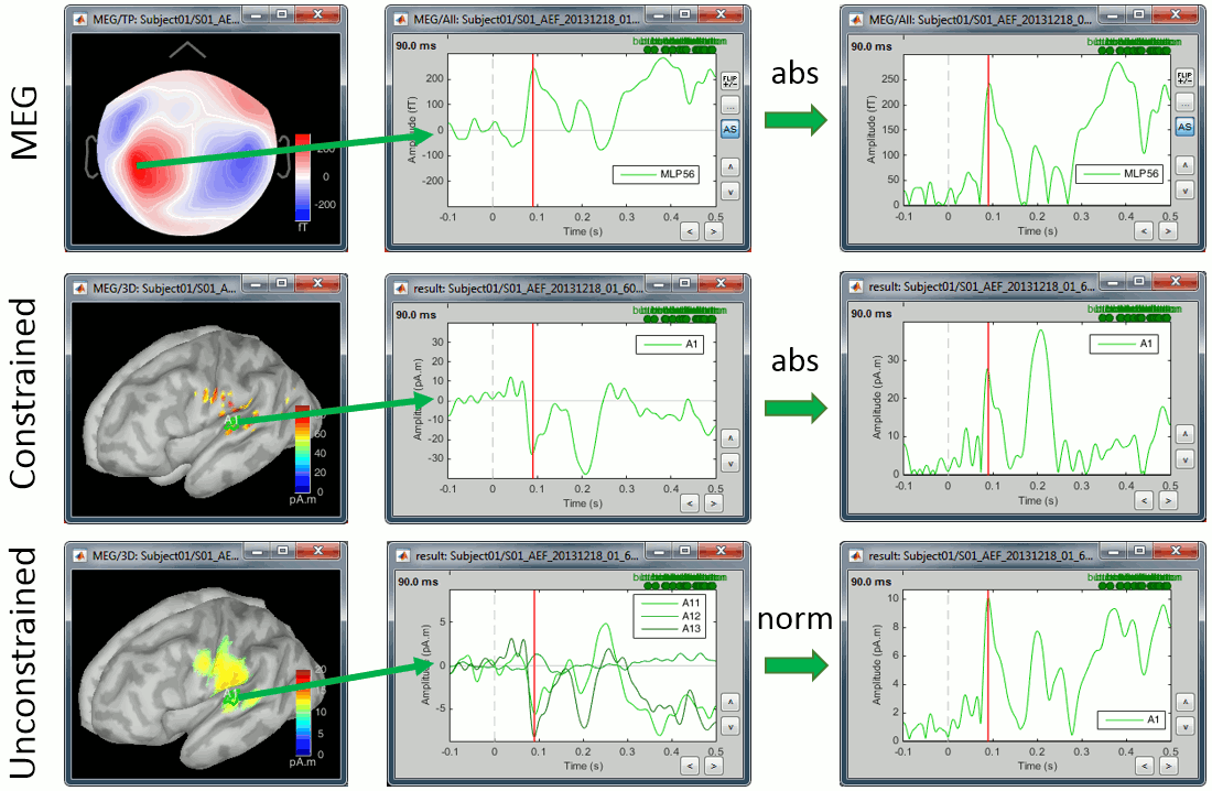
First we need to define on which signals we want to compute the difference: sensor recordings, constrained sources (one signal per grid point) or unconstrained sources (three signals per grid point). For the first two we can compare directly the signals oscillating around zero or their absolute value, for unconstrained sources we have the addional option to compare the norm of the three orientations.

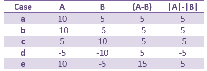
Using the rectified signals (absolute value) give us the an idea of the amount activity in one particular brain region, but alter the frequency information and therefore cannot be used for time-frequency or connectivity analysis. Additionally, the rectified signals are not appropriate to detect effects between different experimental conditions, as illustrated in the next section.

In general, you should not apply an absolute value explicitely to your recordings. The only application cases for rectified signals are the display of the cortical maps (and it is done on the fly) and the comparison of magnitudes between conditions (and then it is done within the process).

Computing a difference

Using sensor recordings or constrained sources:

• Non-rectified (the sign of the difference is ambiguous):
  • Difference of the average current density maps: avg(A) - avg(B)
  • Difference of the Z-score: zscore(avg(deviant)) - zscore(avg(standard))
• Rectified (removing the ambiguity of the sign):
  • Difference of the absolute values of the averages: abs(avg(A)) - abs(avg(B))
  • Difference of the Z-score on absolute values: zscore(avg(A)) - zscore(avg(B))
  • Rectified difference of the averages: (avg(A) - avg(B)) * sign(svg(B))

Using unconstrained sources (three orientations per grid point):

• Difference of the absolute values of the averages: norm(avg(A)) - norm(avg(B))
• Difference of the Z-score: zscore(norm(avg(A))) - zscore(norm(avg(B)))

Sources: Normalized or not

Processing current density maps or normalized source maps do not change these facts, as long as you did not rectify the signals during the computation of the Z-score.

You should be using the Z-score(minnorm) instead of Z-score(abs(minnorm))

Normalize the source maps if you are intending to compare different subjects, it will be help bringing the source maps in the same range of values.

Difference deviant-standard

Before running complicated statistical tests that will take hours of computation, you can start by checking what the difference of the average responses looks like. If in this difference you observe obvious effects that are clearly not what you are expecting, it's not worth moving forward with finer analysis: either the data is not clean enough or your initial hypothesis is wrong.

We are going to use the Process2 tab, at the bottom of the Brainstorm figure. It works exactly like the Process1 tab but with two lists of input files, referred to as FilesA (left) and FilesB (right).

• In Process2, drag and drop the non-normalized deviant average on the left (FilesA) and the non-normalized standard average on the right (FilesB).

• Run the process "Difference > Difference A-B".
  Select the option "Use absolute values", which will convert the unconstrained source maps (three dipoles at each cortex location) into a flat cortical map by taking the norm of the three dipole orientations before computing the difference.
  
  

• Rename the new file in "Deviant-Standard", double-click on it and explore it in time.
  
  

• We are looking at the difference (Deviant-Standard) so positive/red regions indicate higher activity levels for the deviant beeps, and negative/blue regions higher activity for the standard beeps.

  • Before 50ms: The motor activity in the deviant is probably due to the previous stims.

  • P50: Maybe a stronger response in the primary auditory cortex for the standard condition.

  • MMN (125ms): Stronger response for the deviant (left temporal, inferior frontal).

  • 150ms: Stronger response in the auditory system for the standard condition.

  • 175ms: Stronger response in the motor regions for the standard condition (motor inihibition).

  • After 200ms: Stronger response in the deviant condition.

Difference of means

Another process can compute the average and the difference at the same time. We are going to compute the difference of all the trials from both runs at the sensor level. This is usually not recommended because the subject might have moved between the runs. Averaging the recordings across runs is not accurate but can give a good first approximation, in order to make sure we are on the right tracks.

• In Process2, select all the deviant trials (Files A) and all the standard trials (Files B).

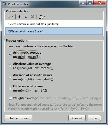
• Run the process "Test > Difference of means", select the option "Arithmetic average".
  
  

• Rename the new file in "Deviant-Standard", double-click on it to display it. The difference deviant-standard does not show anymore the early responses (P50, P100) but emphasizes the difference in the later process (MMN/P200 and P300).
  
  

Parametric Student's t-test [TODO]

Using a t-test instead of the difference of the two averages, we can reproduce similar results but with a significance level attached to each value. Parametric method require the values tested to follow a Gaussian distribution. Some sets of data could be considered as Gaussian (example: screen capture of the histogram of the values recorded by one sensor at one time point), some are not (example: histogram ABS(values) at one point).

WARNING: This parametric t-test is valid only for constrained sources. In the case of unconstrained sources, the norm of the three orientations is used, which breaks the hypothesis of the tested values following a Gaussian distribution. This test is now illustrated on unconstrained sources, but this will change when we figure out the correct parametric test to apply on unconstrained sources.

• In the Process2 tab, select the following files:

  • Files A: All the deviant trials, with the [Process sources] button selected.

  • Files B: All the standard trials, with the [Process sources] button selected.

• Run the process "Test > Student's t-test", Equal variance, Absolute value of average.
  This option will convert the unconstrained source maps (three dipoles at each cortex location) into a flat cortical map by taking the norm of the three dipole orientations before computing the difference.
  
  

• Double-click on the new file for displaying it. With the new tab "Stat" you can control the p-value threshold and the correction you want to apply for multiple comparisons.
  
  

• Set the options in the Stat tab: p-value threshold: 0.05, Multiple comparisons: Uncorrected.
  What we see in this figure are the t-values corresponding to p-values under the threshold. We can make similar observations than with the difference of means, but without the arbitrary amplitude threshold (this slider is now disabled in the Surface tab). If at a given time point a vertex is red in this view, the mean of the deviant condition is significantly higher than the standard conditions (p<0.05).
  
  

• This approach considers each time sample and each surface vertex separately. This means that we have done Nvertices*Ntime = 15002*361 = 5415722 t-tests. The threshold at p<0.05 controls correctly for false positives at one point but not for the entire cortex. We need to correct the p-values for multiple comparisons. The logic of two types of corrections available in the Stat tab (FDR and Bonferroni) is explained in Bennett et al (2009).

• Select the correction for multiple comparison "False discovery rate (FDR)". You will see that a lot less elementrs survive this new threshold. In the Matlab command window, you can see the average corrected p-value, that replace for each vertex the original p-threshold (0.05):
  BST> Average corrected p-threshold: 0.000315138 (FDR, Ntests=5415722)

• From the Scout tab, you can also plot the scouts time series and get in this way a summary of what is happening in your regions of interest. Positive peaks indicate the latencies when at least one vertex of the scout has a value that is significantly higher in the deviant condition. The values that are shown are the averaged t-values in the scout.
  
  

FieldTrip: Non-parametric cluster-based statistic [TODO]

We have the possibility to call some of the FieldTrip functions from the Brainstorm environment. For this, you need first to install the FieldTrip toolbox on your computer and add it to your Matlab path.

For a complete description of non-parametric cluster-based statistics in FieldTrip, read the following article: Maris & Oostendveld (2007). Additional information can be found on the FieldTrip website:

• Tutorial: Parametric and non-parametric statistics on event-related fields

• Tutorial: Cluster-based permutation tests on event related fields

• Tutorial: Cluster-based permutation tests on time-frequency data

• Tutorial: How NOT to interpret results from a cluster-based permutation test

• Video: Statistics using non-parametric randomization techniques

• Video: Non-parametric cluster-based statistical testing of MEG/EEG data

• Functions: ft_timelockstatistics, ft_sourcestatistics, ft_freqstatistics

Permuation-based non-parametric statistics are more flexible and do not require to do any assumption on the distribution of the data, but on the other hand they are a lot more complicated to process. Calling FieldTrip's function ft_sourcestatistics requires a lot more memory because all the data has to be loaded at once, and a lot more computation time because the same test is repeated many times.

Running this function in the same way as the parametric t-test previously (full cortex, all the trials and all the time points) would require 45000*461*361*8/1024^3 = 58 Gb of memory just to load the data. This is impossible on most computers, we have to give up at least one dimension and run the test only for one time sample or one region of interest.

FieldTrip: Process options [TODO]

Screen captures for the two processes:

Description of the process options:

The options available here match the options passed to the function ft_sourcestatistics.

Cluster correction: Define what a cluster is for the different data types (recordings, surface source maps, volume source models, scouts)

Default options:

• clusterstatistic = 'maxsum'
• method = 'montecarlo'
• correcttail = 'prob'

FieldTrip: Example 1 [TODO]

We will run this FieldTrip function first on the scouts time series and then on a short time window.

• Keep the same selection in Process2: all the deviant trials in FilesA, all the standard trials in FilesB.

• Run process: Test > FieldTrip: ft_sourcestatistics, select the options as illustrated below.
  
  

• Double-click on the new file to display it:
  
  

• Display on the cortex: see section "Convert statistic results to regular files" below

FieldTrip: Example 2 [TODO]

short time window

Time-frequency files

Both ft_sourcestatistics and ft_freqstatistics are available.

Use ft_sourcestatistics if the input files contain full source maps, and ft_freqstatistics for all the other cases (scouts or sensors).

Workflow: Single subject

You want to test for one unique subject what is significantly different between two experimental conditions. You are going to compare the single trials corresponding to each condition directly.
This is the case for this tutorial dataset, we want to know what is different between the brain responses to the deviant beep and the standard beep.

Sensor recordings: Not advised for MEG with multiple runs, correct for EEG.

• Parametric t-test: Correct

  • Select the option "Arithmetic average: mean(x)".
  • No restriction on the number of trials.

• Non-parametric t-test: Correct

  • Do not select the option "Test absolute values".
  • No restriction on the number of trials.

• Difference of means:

  • Select the option "Arithmetic average: mean(x)".
  • Use the same number of trials for both conditions.

Constrained source maps (one value per vertex):

• Use the non-normalized minimum norm maps for all the trials (no Z-score).

• Parametric t-test: Incorrect

  • Select the option "Absolue value of average: abs(mean(x))".
  • No restriction on the number of trials.

• Non-parametric t-test: Correct

  • Select the option "Test absolute values".
  • No restriction on the number of trials.

• Difference of means:

  • Select the option "Absolue value of average: abs(mean(x))".
  • Use the same number of trials for both conditions.

Unconstrainted source maps (three values per vertex):

• Parametric t-test: Incorrect

  • ?

• Non-parametric t-test: Correct

  • ?

• Difference of means:

  • ?

Time-frequency maps:

• Test the non-normalized time-frequency maps for all the trials (no Z-score or ERS/ERD).

• Parametric t-test: ?

  • No restriction on the number of trials.

• Non-parametric t-test: Correct

  • No restriction on the number of trials.

• Difference of means:

  • Use the same number of trials for both conditions.

Workflow: Group analysis

You have the same two conditions recorded for multiple subjects.

Sensor recordings: Strongly discouraged for MEG, correct for EEG.

• For each subject: Compute the average of the trials for each condition individually.
  • Do not apply an absolute value.
  • Use the same number of trials for all the subjects.
• Test the subject averages.
  • Do no apply an absolute value.

Source maps (template anatomy):

• For each subject: Average the non-normalized minimumn norm maps for the trials of each condition.
  • Use the same number of trials for all the subjects.

  • If you can't use the same number of trials, you have to correct the Z-score values [TODO].

• Normalize the averages using a Z-score wrt with a baseline.
  • Select the option: "Use absolue values of source activations"
  • Select the option: "Dynamic" (does not make any difference but could be faster).
• Test the normalized averages across subjects.
  • Do not apply an absolute value.

Source maps (individual anatomy):

• For each subject: Average the non-normalized minimumn norm maps for the trials of each condition.
  • Use the same number of trials for all the subjects.

  • If you can't use the same number of trials, you have to correct the Z-score values [TODO].

• Normalize the averages using a Z-score wrt with a baseline.
  • Select the option: "Use absolue values of source activations"
  • Select the option: "Dynamic" (does not make any difference but could be faster).
• Project the normalized maps on the template anatomy.
• Option: Smooth spatially the source maps.
• Test the normalized averages across subjects.
  • Do not apply an absolute value.

Time-frequency maps:

• For each subject: Compute the average time-frequency decompositions of all the trials for each condition (using the advanced options of the "Morlet wavelets" and "Hilbert transform" processes).
  • Use the same number of trials for all the subjects.
• Normalize the averages wrt with a baseline (Z-score or ERS/ERD).
• Test the normalized averages across subjects.
  • Do no apply an absolute value.

Convert statistic results to regular files [TODO]

• Process: Extract > Apply statistc threshold

• Process: Simulate > Simulate recordings from scout [TODO]

Export to SPM

An alternative to running the statical tests in Brainstorm is to export all the data and compute the tests with an external program (R, Matlab, SPM, etc). Multiple menus exist to export files to external file formats (right-click on a file > File > Export to file).

Two tutorials explain to export data specifically to SPM:

• Export source maps to SPM8 (volume)

• Export source maps to SPM12 (surface)

On the hard drive [TODO]

Right click one of the first TF file we computed > File > View file contents.

References

• Bennett CM, Wolford GL, Miller MB, The principled control of false positives in neuroimaging
  Soc Cogn Affect Neurosci (2009), 4(4):417-422.

• Maris E, Oostendveld R, Nonparametric statistical testing of EEG- and MEG-data
  J Neurosci Methods (2007), 164(1):177-90.

• Maris E, Statistical testing in electrophysiological studies
  Psychophysiology (2012), 49(4):549-65

• Pantazis D, Nichols TE, Baillet S, Leahy RM. A comparison of random field theory and permutation methods for the statistical analysis of MEG data, Neuroimage (2005), 25(2):383-94.

• FieldTrip video: Non-parametric cluster-based statistical testing of MEG/EEG data:
  https://www.youtube.com/watch?v=vOSfabsDUNg

Additional discussions on the forum

• Forum: Multiple comparisons: http://neuroimage.usc.edu/forums/showthread.php?1297

• Forum: Cluster neighborhoods: http://neuroimage.usc.edu/forums/showthread.php?2132

• Forum: Differences FieldTrip-Brainstorm: http://neuroimage.usc.edu/forums/showthread.php?2164

Delete all your experiments

Before moving to the next tutorial, delete all the statistic results you computed in this tutorial. It will make it the database structure less confusing for the following tutorials.

---