MEG median nerve tutorial (CTF)

Authors: Francois Tadel, Elizabeth Bock, John C Mosher, Sylvain Baillet

The dataset presented in this tutorial was used in the previous generation of introduction tutorials. We kept it on the website as an additional illustration of data analysis, and as a comparison with median nerve experiments recorded with other MEG systems (Elekta-Neuromag, Yokogawa). No new concepts are presented in this tutorial. For in-depth explanations of the interface and theoretical foundations, please refer to the introduction tutorials.

Download and installation

• Requirements: You have already followed all the basic tutorials and you have a working copy of Brainstorm installed on your computer.

• Go to the Download page of this website, and download the file: sample_raw.zip

• Unzip it in a folder that is not in any of the Brainstorm folders (program folder or database folder).
• Start Brainstorm (Matlab scripts or stand-alone version).

• Select the menu File > Create new protocol. Name it "TutorialRaw" and select the options:

  • No, use individual anatomy,

  • No, use one channel file per run.

Import the anatomy

• Create a new subject Subject01.

• Right-click on the subject node > Import anatomy folder:

  • Set the file format: "FreeSurfer folder"

  • Select the folder: sample_raw/anatomy

  • Number of vertices of the cortex surface: 15000 (default value)

• Click on the link "Click here to compute MNI transformation".

• Set the 3 required fiducial points (indicated in MRI coordinates):
  • NAS: x=127, y=212, z=123
  • LPA: x=55, y=124, z=119
  • RPA: x=200, y=129, z=114

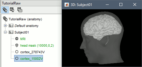
• At the end of the process, make sure that the file "cortex_15000V" is selected (downsampled pial surface, that will be used for the source estimation). If it is not, double-click on it to select it as the default cortex surface.
  
  

Link the recordings

• Switch to the "functional data" view (middle button in the toolbar above the database explorer).

• Right click on the Subject01 > Review raw file:

  • Select the file format: MEG/EEG: CTF

  • Select the folder: sample_raw/Data/subj001_somatosensory_20111109_01_AUX-f.ds

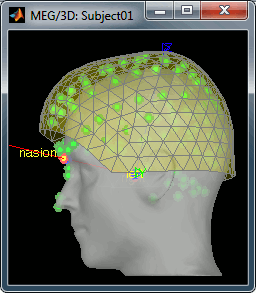
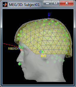
• Refine the registration with the head points: YES.
  
  

Review the recordings

Open the file

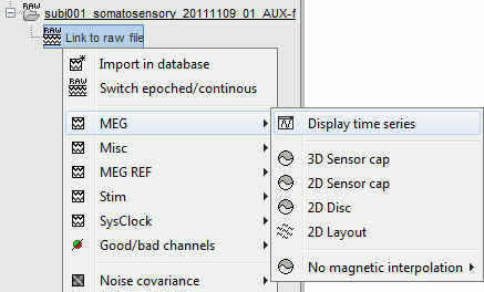
Right-click on the data file > MEG (all) > Display time series.

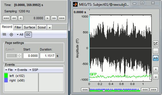
You can see new information in the tab "Record" and a figure showing the recordings.

Identify the unwanted frequencies

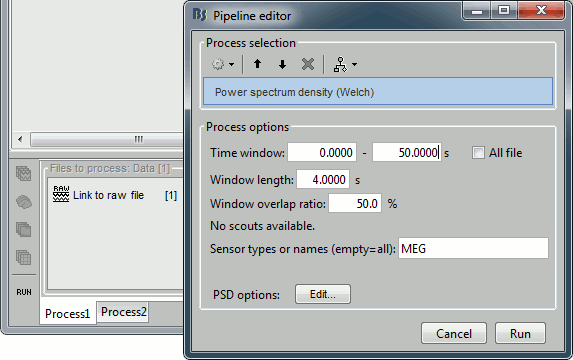
Drag and drop the "Link to raw file" in the Process1 tab, click on the button [Run] to open the Pipeline editor window and select the process "Frequency > Power spectrum density (Welch)". This will estimate the power spectrum of the signal using the Welch method. Set the time window to process to [0,50]s, and the window length to 4 sec, with an overlap of 50%, this will be more than enough to get a good estimate of the spectrum (average of the Fourier transform of 24 windows of 4800 samples each). Leave the other options to the default values.

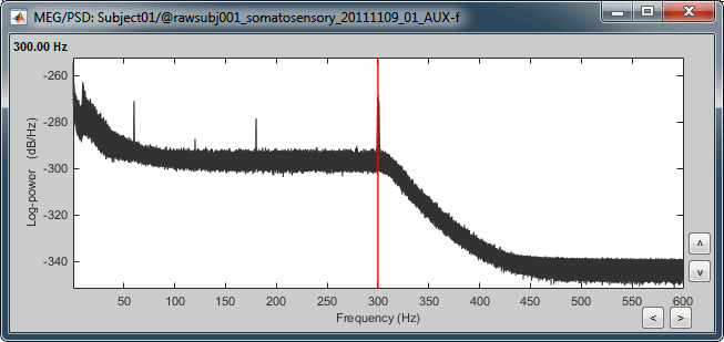
Double click on the "Power (MEG)" file that was created under the "Link to raw file" in the database explorer. This shows the estimate of the power spectrum for the first 50 seconds of the continuous file, for all the sensors, with a logarithmic scale. You can identify four peaks at the following frequencies: 60Hz, 120Hz, 180Hz and 300Hz. The first three are related with the power lines (acquisition in Canada, where the electricity is delivered at 60Hz, plus the harmonics), and are expected to be coming from pure sinusoidal components in the signal. The last one is an artifact of the low-pass filter at 300Hz that was applied on the recordings at the acquisition time. We are going to ignore this one, as it is probably more complex and spanning over several frequency bins.

Remove: 60Hz and harmonics

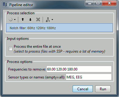
Leave the file "Link to raw file" in the Process1 list and now run "Pre-process > Notch filter".

• Enter the frequencies to remove (60Hz, 120Hz and 180Hz) and leave the other options to the default values.

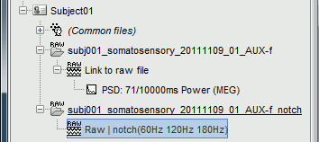
The operation creates a new "Link to raw file" entry in the database, pointing to a new CTF dataset in the same folder as the original continuous file. To check where this file was created: right-click on the file "Raw | notch(60Hz 120Hz 180Hz)" > File > Show in file explorer. This file has the exact same properties as the original file, including the SSP projectors, only the values of the MEG sensors were updated.

Alternatives

If the notch filter is not giving satisfying result, you can use two other processes:

• Sinusoid removal: This process can do a better job at removing precise frequencies by identifying the sinusoidal components and then subtracting them from the signals in time domain (not a frequency filter).

• Band-stop filter: This process can be useful for removing larger segments of the spectrum, in case the power line peaks are spread over numerous frequency bins or for suppressing other types of artifacts.

Evaluate the results

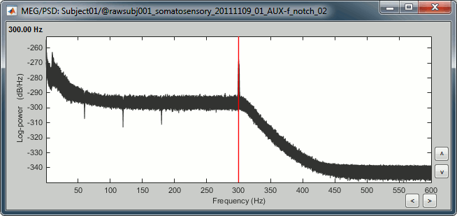
Now run the same frequency analysis: process "Frequency > Power spectrum density (Welch)", time window = [0,50]s, window length = 4000ms, overlap = 50%. Double click on the new "Power (MEG)" file. As expected, the three first peaks due to the power lines are gone.

You can run a few other pre-processing operations directly on the continuous files, including a band-pass filter. Frequency filters and sinusoid removals are operations that you should apply at very early stages of the analysis, before epoching the recordings. These operations do not perform well next to the beginning and the end of the signals, they may generate important artifacts. It is therefore much more accurate to filter the entire recordings from the original continuous file at once, rather than filtering small epochs after importing them in the database.

From now on, we are only going to work on this clean file "Raw | notch(60Hz 120Hz 180Hz)".

Signal Space Projection

The Signal-Space Projection (SSP) is one approach to rejection of external disturbances. Here is a short description of the method by Matti Hämäläinen, from the MNE 2.7 reference manual, section 4.16.

Unlike many other noise-cancellation approaches, SSP does not require additional reference sensors to record the disturbance fields. Instead, SSP relies on the fact that the magnetic field distributions generated by the sources in the brain have spatial distributions sufficiently different from these generated by external noise sources. Furthermore, it is implicitly assumed that the linear space spanned by the significant external noise patterns has a low dimension.

Without loss of generality we can always decompose any n-channel measurement b(t) into its signal and noise components as:

• b(t) = b_''s''(t) + b_''n''(t)

Further, if we know that b_''n''(t) is well characterized by a few field patterns b_''1''...b_''m'', we can express the disturbance as

• b_''n''(t) = Uc_''n''(t) + e(t) ,

where the columns of U constitute an orthonormal basis for b_''1''...b_''m'', c_''n''(t) is an m-component column vector, and the error term e(t) is small and does not exhibit any consistent spatial distributions over time, i.e., C_''e'' = E{ee^''T''} = I. Subsequently, we will call the column space of U the noise subspace. The basic idea of SSP is that we can actually find a small basis set b_''1''...b_''m'' such that the conditions described above are satisfied. We can now construct the orthogonal complement operator

• P_⊥ = I - UU^T

and apply it to b(t) yielding

• b(t) ≈ P_⊥b_''s''(t) ,

since P_⊥b_''n''(t) = P_⊥Uc_''n''(t) ≈ 0. The projection operator P_⊥ is called the signal-space projection operator and generally provides considerable rejection of noise, suppressing external disturbances by a factor of 10 or more. The effectiveness of SSP depends on two factors:

1. The basis set b_''1''...b_''m'' should be able to characterize the disturbance field patterns completely and

2. The angles between the noise subspace space spanned by b_''1''...b_''m'' and the signal vectors b_''s''(t) should be as close to π/2 as possible.

If the first requirement is not satisfied, some noise will leak through because P_⊥b_''n''(t) ≠ 0. If the any of the brain signal vectors b_''s''(t) is close to the noise subspace not only the noise but also the signal will be attenuated by the application of P_⊥ and, consequently, there might by little gain in signal-to-noise ratio.

Since the signal-space projection modifies the signal vectors originating in the brain, it is necessary to apply the projection to the forward solution in the course of inverse computations.

For more information on the SSP method, please consult the following publications:

• C. D. Tesche, M. A. Uusitalo, R. J. Ilmoniemi, M. Huotilainen, M. Kajola, and O. Salonen, "Signal-space projections of MEG data characterize both distributed and well-localized neuronal sources," Electroencephalogr Clin Neurophysiol, vol. 95, pp. 189-200, 1995.
• M. A. Uusitalo and R. J. Ilmoniemi, "Signal-space projection method for separating MEG or EEG into components," Med Biol Eng Comput, vol. 35, pp. 135-40, 1997.

Identify the artifacts

The first step is to identify several repetitions of the artifact (the vectors b_''1''...b_''m''). We need to set markers in the recordings that indicate when the events that we want to correct for occur. To help with this task, it is recommended to always record with bipolar electrodes the activity of the eyes (electro-oculogram or EOG, vertical and horizontal), the heart (electro-cardiogram or ECG), and possibly other sources of muscular contaminations (electromyogram or EMG). In this example, we are going to use the ECG and vertical EOG traces to mark the cardiac activity and the eye blinks. Two methods can be used, manual or automatic.

EOG/ECG channels

• Select the protocol TutorialRaw created in the previous tutorial, and select the "Functional data" view (second button in the toolbar on top of the database explorer).

• Double-click on the clean continuous recordings ("Raw | notch(60Hz 120Hz 180Hz)") to open the MEG recordings.

• Set the length of the reviewed time window to 3 seconds (in the Record tab, text box "Duration")

• Right-click on the continuous recordings again > Misc > Display time series.

  • 

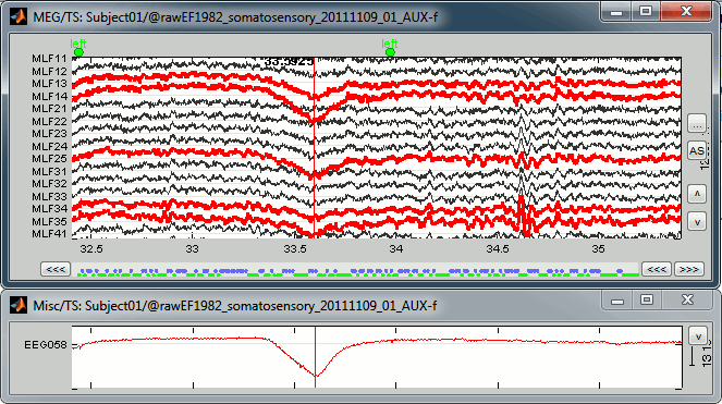
• In this file the channel type "Misc" groups the two channels EEG057 (ECG, in green) and EEG058 (vertical EOG, in red). This configuration depends on the acquisition setup, and can be redefined afterwards in Brainstorm (right-click on the channel file > Edit channel file, and then change manually the string in the column Type for any channel).

• Use the shortcuts introduced in the previous tutorial to adjust the vertical scale of this display: Shift+mouse wheel, +/- keys, or the buttons on the right side of the figure.

• Then go further in time to see what is happening on these channels over the time: use the ">>>" buttons, or the associated shortcuts (read the tooltips of the button)

• ECG: On the green trace, you can recognize the very typical shape of the electric activity of the heart (P, QRS and T waves). This is a very good example, the signal is not always that clean.

• EOG: On the red trace, there is not much happening for most of the recordings except for a few bumps, typical of eye blinks, eg. at 33.590s. This subject is sitting very still and not blinking much. We can expect MEG recordings of a very good quality.

• You can observe the contamination from a blink on the left-frontal sensors: move to 33.590s (you can use the text boxes in the time panel, the Record tab, or the scrollbar in the figure), and select a subset of sensors (Shift+B, or right-click on the figure > Display setup > CTF LF)

  • 

Manual marking

Create a new category of markers "blink_manual", using the menu Events > Add group. Select this new group. Review the file, and mark the peaks you observe on the vertical EOG trace, using the Ctrl+E keyboard shortcut. Do that for a few eye blinks.

You could repeat the same operation for all the blinks, then for all the ECG peaks and jump to the next chapter of the tutorial and compute the SSP. It would be uselessly time consuming, as there is a process that does it for you automatically. However, it is good to remember how to do it manually because you may face some cases where you don't have clean ECG/EOG, or if you want to correct for another type of artifact.

Automatic detection: EOG

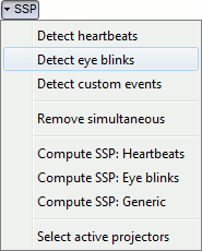
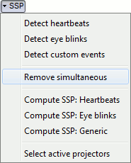
In the Record tab, select the menu: SSP > Detect eye blinks. It automatically opens the pipeline editor, with the process "Detect eye blinks" selected:

• Channel name: Name of the channel that is used to perform the detection. Select or type "EEG058" as it is the name of the EOG channel

• Time window: Time range that the algorithm should scan for the selected artifact. Leave the default values to process the entire file.

• Event name: Name of the event group that is created for saving all the detected events. Leave the default "blink".

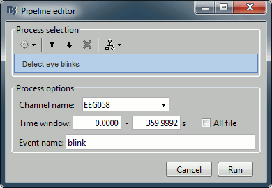
Click on Run. After the process stops, you can see two new event categories "blink" and "blink2" in the Record tab. You can review a few of them, to make sure that they really indicate the EOG events. In the Record tab, click on the "blink" event category, then on a time occurrence to jump to it in the MEG and Misc time series figures.

Two types of events are created because this algorithm not only detects specific events in a signal, it also classifies them by shape. If you go through all the events that were detected in the two categories, you would see that the "blink" are all round bumps, typical of the eye blinks. In the category "blink2", the morphologies don't look as uniform; it mixes small blinks, and ramps or step functions followed by sharp drops that could indicate eye saccades. The saccades can be observed on the vertical EOG, but if you want a better characterization of them you should also record the horizontal EOG. The detection of the saccades should be performed with a different set of parameters, using the process "Detect custom events", introduced later in this chapter.

Automatic detection: ECG

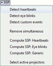
Now do the same thing for the heartbeats. In the Record tab, select the menu "SSP > Detect heartbeats". Configure the process to use the channel EEG057 (name of the ECG channel), and leave the other options to the default values.

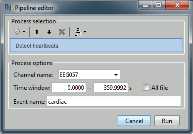
Click on Run. After the process stops, you can see a new event category "cardiac" in the Record tab, with 346 occurrences. You can check a few of them, to make sure that the "cardiac" markers really indicate the ECG peaks, and that there are not too many peaks that are skipped.

Automatic detection: Custom

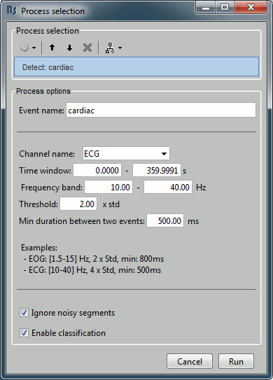
These two previous processes are shortcuts for a generic process "Detect custom events". We are not going to use it here, but it is interesting to introduce it to understand how the blinks and heartbeats detection work. The logic is the following:

• The channel to analyze is read from the continuous file, for a given time window.

• Frequency band: The signal is filtered in a frequency band where the artifact is easy to detect. For EOG: 1.5-15Hz ; for ECG: 10-40Hz.

• Threshold: An event of interest is detected if the absolute value of the filtered signal value goes over a given number of times the standard deviation. For EOG: 2xStd, for ECG: 4xStd

• Minimum duration between two events: If the filtered signal crosses the threshold several times in relation with the same artifact (like it would be the case for muscular activity recordings on an EMG channel), we don't want to trigger several events but just one at the beginning of the activity. This parameter would indicate the algorithm to take only the maximum value over the given time window; it also prevents from detecting other events immediately after a successful detection. For the ECG, this value is set to 500ms, because it is very unlikely that the heart rate of the subject goes over 120 beats per minute.

• Ignore the noisy segments: If this option is selected, the detection is not performed on the segments that are much noisier than the rest of the recordings.

• Enable classification: If this option is selected, the events are classified by shape, based on correlation measure. In the end, only the categories that have more than 5 occurrences are kept, all the other successful detections are ignored.

Calculate the projectors

Methodology

We have now 346 examples of heartbeats, 18 examples of blinks, and 12 examples of saccades. These are sufficient numbers of repetitions to calculate reliable signal-space projections. The logic of the computation is the following:

1. Take a small time window around each marker to capture the full effect of the artifact, plus some clean brain signals before and after. The default time window is [-200,+200]ms for eye blinks, and [-40,+40]ms for the heartbeats.
2. Filter the MEG or EEG signals in a frequency band of interest, in which the artifact is the most visible.

3. Concatenate all these time blocks into a big matrix A = [b_''1'', ..., b_''m'']

4. Compute the singular value decomposition of this matrix A: [U,S,V] = svd(A, 'econ')

5. The singular vectors Ui with the highest singular values Si are an orthonormal basis of the artifact subspace that we want to subtract from the recordings. The software selects by default the first vector only but it is possible to redefine interactively the selected components.

6. Calculate the projection operator: P_⊥i = I - UiUi^T

7. Apply this projection on the MEG or EEG recordings F: F = P_⊥iF

8. The process has to be repeated separately several times:

   • for each sensor type (EEG, MEG magnetometers, MEG gradiometers) and
   • for each artifact, starting with the one that leads to the strongest contamination in amplitude on the sensors (in the case: the eye blinks)
   • If you have difficulties removing one artifact or the other, you may try to process them in a different order. You may also try removing some of the artifact markers in the case of co-occurring artifacts. If a lot of the blinks happen at the same time as heartbeats, you may end up calculating projectors that mix both effects, but that do not remove efficiently one or the other. In this case, remove all the markers that happen in the segments contaminated by multiple artifacts.

Steps #1 to #5 are automatically done by the processes "SSP > Compute SSP" in the Record tab: the results, the vectors Ui, are saved in the database link ("Link to raw file") and in the channel file.

Steps #6 and #7 are calculated on the fly when reading a block of recordings from the continuous file: when using the raw viewer, running a process a process on the continuous file, or importing epochs in the database.

Step #8 is the manual control of the process. Take some time to understand what you are trying to remove and how to do it. Never trust blindly any fully automated artifact cleaning algorithm, always check manually what is removed from the recordings, and do not give up if the first results are not satisfying.

Recommended procedure

We have multiple types of artifact to correct for and it can be tricky to know what artifact to correct first. If you correct for artifact A and then for artifact B, you may get different results than if you correct first B and then A. We propose here a default order for the two artifacts that we have in all the recordings: the blinks and the heartbeats.

If two artifacts happen at the same time, the SSP projectors calculated for the blink may contain some of the heartbeat and vice versa. When trying to remove the second artifact, we might not be able to isolate it clearly anymore. To avoid this behavior, we should try to avoid having overlapping artifacts. Because the subject's heart is beating at least once per second, there is a high chance to record a heartbeat next to any eye blink. Therefore a significant number of the blinks will be contaminated with heartbeats. If we decide to remove all the blink events that include some heart activity, we may not have enough blink samples left to build correct SSP projectors. To isolate correctly these two common contaminations we recommend the following procedure:

1. Remove all the cardiac peaks that are occurring next to a blink (we can remove half of the heartbeats, we will still have enough data for calculating the projectors).

2. Calculate the SSP to remove the cardiac artifact.

3. Calculate the SSP to remove the eye blinks, based on the recordings already corrected for the cardiac artifact.

Remove simultaneous events

If you closed the file viewer, open the MEG recordings again:

• double click on the clean file "Raw | notch(60Hz 120Hz 180Hz)".

In the Record tab, select the menu "SSP > Remove simultaneous". Set the options:

• Remove events named: "cardiac"

• When too close to events: "blink"

• Minimum delay between events: 250ms

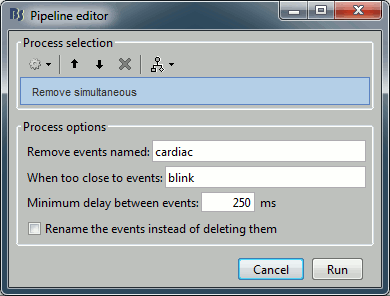
After executing this process, the number of "cardiac" events goes from 346 to 333. The deleted heartbeats were all less than 250ms away from a blink.

Compute SSP: Heartbeats

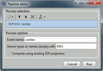
In the Record tab, select the menu "SSP > Compute SSP: Heartbeats". Set the options:

• Event name: Name of the event to use to calculate the projectors, enter "cardiac"

• Sensor types: Type of sensors for which the projection should be calculated ("MEG"). It doesn't matter if there are other sensor types indicated in the text box: the sensor names or types that do not exist in the recordings are just ignored. Note that you will always get better results if you process the different types of sensors separately. If you have MEG and EEG in the same file, you should run twice this process, once for the EEG only and once for the MEG only. Same thing when processing Elekta-Neuromag recordings, you should process separately the magnetometers (MEG MAG) and the gradiometers (MEG GRAD).

• Compute using existing SSP projectors: You have the option to calculate the projectors from the raw recordings, or from the recordings filtered with the previously computed SSP projectors. Unless you have a good reason for not considering the existing SSP projectors, you should always select this option.

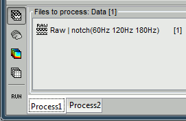
After the computation is done, a new figure is displayed, that lets you select the active projectors. On the left you have the projector categories (matrix U) where each row represents the result of an execution of a "Compute SSP " process (usually one for each sensor type and each artifact). On the right, you can activate independently the different components for the selected projector category. Each entry represents the projector created from a column vector Ui (singular vector of the SVD decomposition), and the percentage is the singular value for this vector, normalized for this decomposition (percentage = Si / sum(Si)). When a projector is selected, it means that it is applied to the recordings on the fly when reading from the continuous file, ie. that the corresponding spatial component is removed from the recordings.

The percentage indicates the amount of signal that was captured by this projector during the decomposition. The highest it is, the more the projector is representative of the artifact recordings that were used to calculate it. In the good cases, you would typically see one to three components with values that are significantly higher that the others.

By default, the software selects the first component and leaves all the others unselected. Do not trust this automatic selection, you should always review manually the components that you want to remove.

A list of buttons is available to manipulate the projector categories: load, save, rename, delete, and display component topography. The last one is one of the most useful tool to understand these results. Select the category ("cardiac"), click on the first component, then click on the toolbar button to display its topography. Do it again for components #2 and #3 (the components don't need to be active for that).

The other button [No interp] displays the same results without the magnetic field smoothing that is applied by default to MEG topographies. It may help understand some difficult cases.

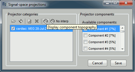
None of these topographies can be clearly related to a cardiac component. This can have two interpretations: the cardiac artifact is not very strong for this subject and the influence of the heart activity over the MEG sensors is completely buried in the noise or the brain signals, or the characterization of the artifact that we did was not so good and we should refine it by selecting for instance smaller time windows around the cardiac peaks. Here, it's probably due to the subject's morphology. Some people generate strong artifacts in the MEG, some don't.

In this case, it is safer to unselect this "cardiac" category, rather than removing randomly spatial components that we are not sure to identify.

Compute SSP: Eye blinks

Let's try the same thing with the eye blinks. Select the process "SSP > Compute SSP: Eye blinks". Run it on the event type "blink", that indicate the peaks of the EOG signal.

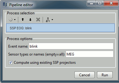
In this specific case, there is one value that is much higher than the others (21%). The first component is most likely a good representation of the artifact we are trying to remove.

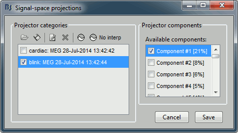
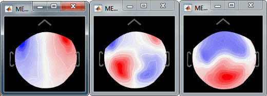
Select the cardiac category, and display the topographies for the first three components. Component #1 is clearly related with the ocular activity occurring during the blinks, the others are not as clear. Conclusion: the default proposition was good (only component #1 selected). Setting this first projector as active removes from the MEG signals the contributions related with the spatial topography we can see in the first figure, ie. a spatial distribution of sensor values related specifically to the eye blinks.

While the recordings are displayed in the file viewer, the selection of the active projectors interactively updates the recordings. Go to the first detected "blink" event (t=33.600s), and select the left frontal sensors (Shift+B or right-click > Display setup > CTF LF). Then play with the checkboxes to change the active projectors, and see how well this first component of the blink category removes the ocular artifact.

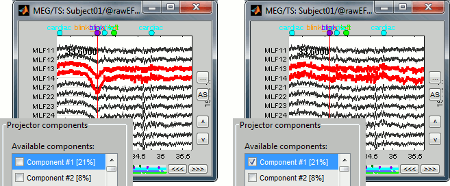
Select the projector category "blink", select the first component, and click on Save, to validate your changes. Starting from now, all the successive operations you apply on this file will integrate this eye blink correction, including the calculation of other projectors. After you closed this window, you can get back to it by selecting the menu "SSP > Select active projector" in the Record tab, and change again the selection of active projectors.

We are not going to calculate the SSP for the other category of events identified on the EOG, the group "blink2". The events classified in this group could represent eye saccades or other types of blinks, it is not very clear that they correspond to the same physiological event. Most of them do not seem to create any obvious contamination on the MEG recordings, there is probably no need to consider them now.

Compute SSP : Generic

The calculation of the SSP for the heartbeats and the eye blinks are shortcuts to a more generic algorithm "Compute SSP: Generic". We do not need it here, but the illustration of its properties is interesting to understand the correction of ocular and cardiac artifacts:

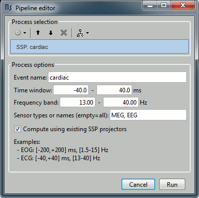
• Event name: Markers that are used to characterize the artifact

• Time window: Time segment to consider before and after each event marker. We want this time window to be longer than the artifact effect itself, in order to have a large number of time samples representative of a normal brain activity. This helps the SVD decomposition to separate the artifact from the ongoing brain activity.

• Frequency band: Definition of the band-pass filter that is applied to the recordings before calculating the projector. Usually you would use the same frequency band as we used for the detection, but you may want to try to refine this parameter if the results are not satisfying.

• Sensor types or names: List of sensors for which to calculate the projector. You can get better results if you process one sensor type at a time.

Troubleshooting

You have calculated the SSP as indicated here but you don't get any good results. No matter what you do, the topographies don't look like the targeted artifact. You can try the following:

• Review one by one the events indicating the artifacts, remove the ones that are less clear or that occur close to another artifact.
• Select or unselect the option "Compute using existing SSP".
• Use the process "Compute SSP: Generic" and modify some parameters:
  • Reduce the time window around the peak of the artifact.
  • Use a narrower frequency band: especially the EOG, if the projectors capture some of the alpha oscillations, you can limit the frequency band to [1.5 - 9] Hz.
  • Change the method: Average / SSP.
• If you have multiple acquisition runs, you may try to use all the artifacts from all the runs rather than processing the files one by one. For that, use the Process2 tab instead of Process1. Put the "Link to raw file" of all the runs on both side, Files A (what is used to compute the SSP) and Files B (where the SSP are applied).

Evaluation

Eye blinks

One efficient way of representing the impact of this artifact correction is to epoch the recordings around the artifacts before and after the correction. Use the same time window as the one used in the SSP options around each marker, and average all the segments of recordings. These operations are detailed in the next tutorial, we are just presenting the results. You don't need to reproduce them at this time, just remember that it is doable, in case you need it with your own data. This is what the database would look like after these operations:

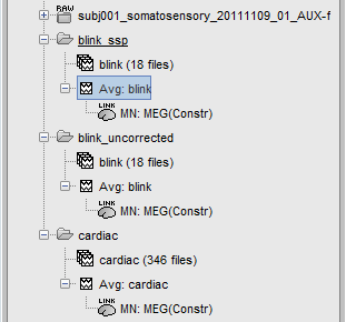
The following image represents the file "blink_uncorrected / Avg: blink", which is the average of the 18 identified blinks before the SSP correction, [-200,+200]ms around the "blink" events. The time series, the 2D topography at the peak (t = 0ms), and the mapping on the cortex of these fields, using the basic inverse model calculated in the previous tutorial.

The next image represents the file "blink_ssp / Avg: blink", which is the exact same thing, but after the SSP correction. The artifact is gone. If you do this and you can still see some clear evoked component in the time series figure, the SSP correction was not efficient: the artifact is not properly identified, or you should select different components using the "Select active projectors" window.

Heartbeats

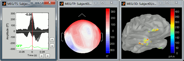
We can do the same thing with the heartbeats: epoch [-40,+40]ms around the "cardiac" events, average the trials, and review the event-related fields at three instants:

The peak of the P wave (t = -30ms):

The peak of the QRS complex (t = 0ms):

The peak of the T wave (t = 25ms):

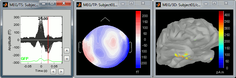
These peaks may look big, but they are in fact much smaller (300 fT for the average of 346 repetitions) than what we observed for the eye blinks (1500 fT for 18 repetitions). You can notice that none of these topographies are similar to the components we obtained after calculating the SSP for the cardiac artifact. We don't know how to correct this artifact, it doesn't look too bad in terms of recordings contamination, so we just leave it uncorrected.

C3. Epoching and averaging

Authors: Francois Tadel, Elizabeth Bock, John C Mosher, Sylvain Baillet

This tutorial fills the gap between the previous tutorial (review and clean continuous recordings), and the introduction tutorials (source analysis of evoked responses). It explains how to epoch the recordings, do some more pre-processing on the single trials, and then calculate their average. For this tutorial, we are going to use the protocol TutorialRaw created in the two previous tutorials: Review continuous recordings and edit markers and Artifact cleaning. If you have not followed these tutorials yet, please do it now.

Import in database

The raw file viewer provides a rapid access to the recordings, but most of operations cannot be performed directly on the continuous files: most of the pre-processing functions, averaging, time-frequency analysis and statistical tests can only be applied on blocks of data that are saved in the database (ie. "imported"). After reviewing the recordings and editing the event markers, you have to "import" the recordings in the database to go with further analysis.

Right-click on the file with power line correction: Raw | notch(60Hz 120Hz 180Hz) > Import in dabase

Warning: If you right-click on the subject node > Import EEG/MEG, and select the tutorial .ds dataset, you would be able to import blocks of the continuous file in the database, but you would not have access to the modified events list or the SSP operators. Therefore, you would not import data cleaned of ocular and cardiac artifacts. The modified events list and the signal space projectors are saved only in the "Link to raw file" in the Brainstorm database, not in the initial continuous file.

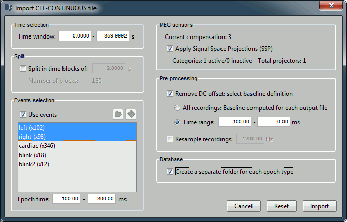
Set the import options as they are represented in this figure:

• Time window: Time range of interest. We are interested by all the stimulations, so do not change this parameter; the default values always represent the entire file.

• Split: Useful to import continuous recordings without events, to import successive chunks of the same duration. We do not need this here.

• Events selection: Check the "Use events" option, and select both "left" and "right". The number in the parenthesis represents the number of occurrences of this event in the selected time window (would change if you modify the time definition on top of the figure)

• Epoch time: Time segment that is extracted around each marker and saved in the database. Set it to [-100, +300] ms

• Use Signal Space Projections: Use the active SSP projectors calculated during the previous pre-processing steps. Keep this option selected.

• Remove DC Offset: Check this option, and select: Time range: [-100, 0] ms. For each epoch, this will: compute the average of each channel over the baseline (pre-stimulus interval: -100ms to 0ms), and subtract it from the channel at every time instants (full epoch interval: [-100,+300]ms). This option removes the baseline value of each sensor, ie. the continuous (DC) offset that is added permanently on top of the recordings of interest. In MEG, the sensors record variations around a somewhat arbitrary level, therefore this operation is always needed, unless it was already applied during one of the pre-processing steps. Note that a high-pass filter with a very low frequency (for instance 0.3Hz) can replace efficiently this DC correction. If a high-pass filter has already been applied to the recordings, you may want to unselect this option.

• Resample recordings: Keep this unchecked

• Create a separate folder for each epoch type: If selected, a new folder is created for each event type (here, it will create two folders in the database: "left" and "right"). If not selected, all the epochs are saved in a new folder, the same one for all the events, that has the same name as the initial raw file.

Click on Import and wait. At the end, you are asked whether you want to ignore one epoch that is shorter than the others. This happens because the acquisition of the MEG signals was stopped less than 300ms after the last stimulus trigger was sent. Therefore, the last epoch cannot have the full [-100,300]ms time definition. This shorter epoch would prevent us from averaging all the trials easily. As we already have enough repetitions in this experiment, we can just ignore it. Answer Yes to this question to discard the last epoch.

Two new conditions containing two groups of trials appeared in the database. To expand a group of trials and get access to the individual epochs: double-click on it or click on the "+" next to it.

The SSP projectors calculated in the previous tutorial were applied on the fly when reading from the continuous file. These epochs are clean from eye blinks and power line contamination.

All the files available in the (Common files) folder are also shared for these new folders "left" and "right".

Review the individual trials

Double-click on the first trial for the "left" condition. Then right-click on the figure > Navigator > Next data file, or use the keyboard shortcut F3 to jump to the next trial. This way you can quickly review all the trials, to make sure that there is no obvious problem in the recordings. If you haven't reviewed manually all the recordings in the continuous mode, and marked all the bad segments, it is a good time to do it now.

To mark a trial as bad manually, you have three methods:

• Right-click on the trial file in the database > Reject trial

• Right-click on the figure > Reject trial

• Use the keyboard shortcut Control+B

• To set all the trials back as good in a group: right-click on the trials group or the condition > Accept bad trials.

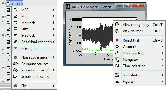
When a trial is tagged as bad, its icon in the database explorer shows a red mark.

All the bad trials are going to be ignored in the rest of the analysis, because they are ignored by the Process1 and Process2 tabs. If you drag and drop the 101 left trials in the Process1 list, with one trial marked as bad, the summary of the selected files on top of the tab would show only 100 data files.

To learn how to mark only individual channels as bad instead of the entire trial, please go back to the introduction tutorial Exploring the recordings.

The process "Artifacts > Detect bad channels: peak-to-peak" can help you detect some bad trials based on a peak-to-peak amplitude threshold. Drag and drop all the trials from the left condition in the Process1 list, and select this process. For each trial, it detects the channels that have a peak-to-peak amplitude (maximum value - minimum value) that is above a rejection threshold (too noisy) or below a rejection threshold (no signal). You can define different thresholds for different channel types. The options are:

• Time window: Time range on which the peak-to-peak amplitude is calculated on each trial

• Thresholds: Rejection and detection thresholds for each sensor type. For CTF recordings, use the "MEG gradio" category, and ignore the "/cm (x 0.04)" indication, that is valid only for Neuromag systems. Set the MEG gradio thresholds to [0, 2000] fT, to detect the MEG channels that have a peak-to-peak amplitude superior to 2000fT.

• Reject only the bad channels: This would tag as bad only the detected channels, but would not tag the trial itself as bad.

• Reject the entire trial: This would tag as bad the trial if there is at least one channel file identified as bad.

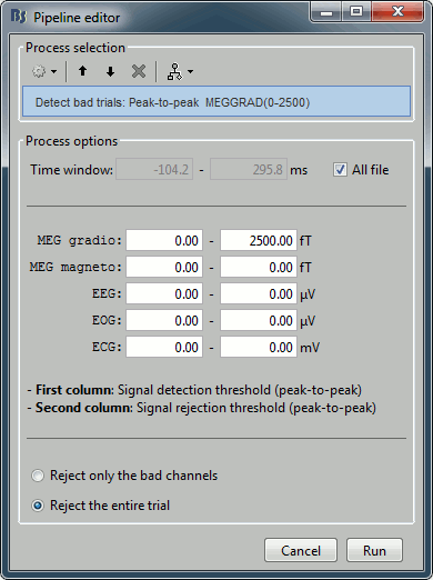
For this current dataset, the quality of the recordings is remarkably good, we don't need to mark any trial as bad. So right-click on the group of "left" trials > Accept trials, to set them all as good.

Averaging

Drag and drop the two lists of trials (or the two condition folders) in the Process1 list, and run the process "Average > Average files", with the option "Average by condition (subject average)". This will group the trials by conditions, and calculate one average per condition and subject. The option "By condition (grand average)" would average each condition for all the subjects together, but as there is only one subject in this case, the result would be same. The other options would generate one average file per subject ("by subject"), one average file per group of trials and per subject ("by trial group"), or only one average no matter what the input is ("everything").

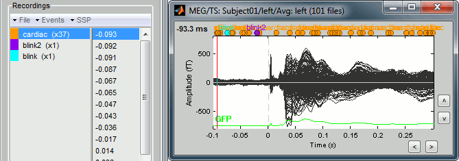
The function to apply is the regular arithmetic average. The option "Keep all the events from the individual epochs" would group all the event markers present in all the epochs and save them in the new averaged file. It can be useful to check the relative position of the artifacts or the subject responses, or quickly detect some unwanted configuration such as a subject who would constantly blink right after a visual stimulus. We don't really need this here, leave this option unselected.

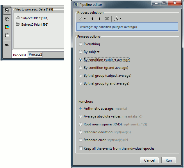
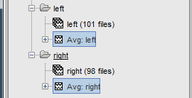
It creates two files: "Avg: left" and "Avg: right".

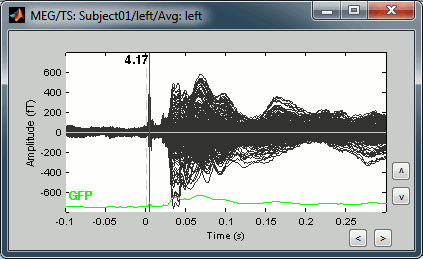
Double-click on the "Avg: Left" file to display the MEG recordings for this file (or right-click > MEG > display time series). It shows a very typical an clean evoked response, with a very high signal-to-noise ratio.

Just for the records, this is how it would look like if we had selected the option "Keep all the events from the individual epochs". The summary of the markers of all the epochs is: 37 heartbeats and 2 blinks.

Stimulation artifact

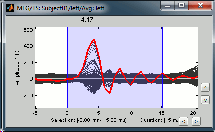
Now zoom around 4ms in time (mouse wheel, or two figures up/down on macbooks) and amplitude (control + zoom). Notice this very strong and sharp peak followed by fast oscillations. This is an artifact due to the electric stimulation device. In the stimulation setup: the stimulus trigger is initiated by the stimulation computer and sent to the electric stimulator. This stimulator generates an electric pulse that is sent to electrodes on the subject's wrists. This electric current flows in the wires and the in the body, so it also generates a small magnetic field that is captured by the MEG sensors. This is what we observe here at 4ms.

This means that whenever we decide to send an electric stimulus, there is a 4ms delay before the stimulus is actually received by the subject, due to all the electronics in between. Which means that everything is shifted by 4ms in the recordings. These hardware delays are unavoidable and should be quantified precisely before starting scanning subjects or patients.

Then you have two options: either you remember it and subtract the delays when you publish your results (there is a risk of forgetting about them), or you fix the files right now by fixing the time reference in all the files (there is a risk of forgetting to fix all the subjects/runs in the same way). Let's illustrate this second method now.

Close all the figures, clear the Process1 list (right-click > clear, or select+delete key), and drag and drop all the trials and all the averages (or simply the two left and right condition folders). Select the process "Pre-process > Add time offset". Set the time offset to -4.2 ms, to bring back this stimulation peak at 0ms. Select also the "Overwrite input files" option, to avoid too many duplications of unnecessary files in the database.

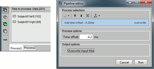
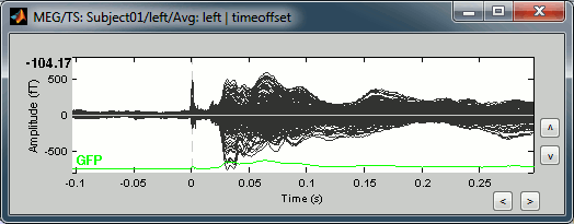
This fixes the individual trials and the averages. Double-click on the "Avg: left" file again to observe that the stimulation artifact is now occurring at 0ms exactly, which means that t=0s represents the time when the electric pulse is received by the subject.

Filters for visualization

As introduced in the previous tutorials, you can add a visualization filter to make the traces and the topographies look smoother. We suggest in this case a low-pass filter at 120Hz, because it shows very smooth traces, but all the waves we are interested in are still clearly visible in the MEG time series figure.

Explore the average

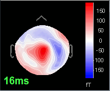
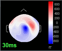
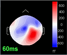
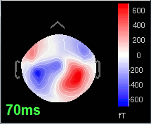
Open the time series for the "Avg: left". Then press Control+T, to see on the side a spatial topography at the current time point. Then observe what is happening between 0ms and 100ms. Start at 0ms and play it like a movie using the arrow keys left and right, to follow the brain activity millisecond by millisecond:

• 16 ms: First response, the sensory information reaches the right somatosensory cortex (S1)

• 30 ms: Stronger and more focal activity in the same region, but with a source oriented in the opposite direction (S1)

• 60 ms: Activity appearing progressively in a more lateral region (S1 + S2)

• 70 ms: Activity in the same area in the left hemisphere (S2 left + S2 right)

Source analysis

Let's reproduce the same observations at the source level. The concepts related with the source estimation are not discussed here; for more information, refer to the introduction tutorials #6 to #8.

First, delete all the files related with the source estimation calculated in the previous tutorials, available in the (Common files) folder: the head model, the noise covariance and inverse model. We can now provide a better estimate of the noise (affects the inverse model), and we defined new SSP operators (affects the head model).

Head model

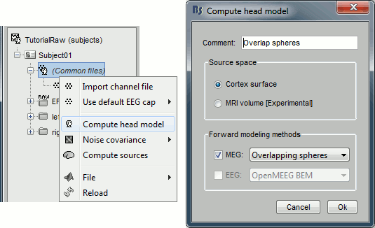
Right-click on any node that contains the channel file (including the channel file itself), and select: "Compute head model". Leave all the default options: cortex source space, and overlapping spheres. The lead field matrix is saved in file "Overlapping spheres" in (Common files).

Noise covariance matrix

To estimate the sources properly, we need an estimation of the noise level for each sensor. A good way to do this is to compute the covariance matrix of the concatenation of the baselines from all the trials in both conditions.

• Select at the same time the two groups of trials (right and left). To do this: hold the Control (or Cmd on Macs) key and click successively on the Right and the Left trial lists.

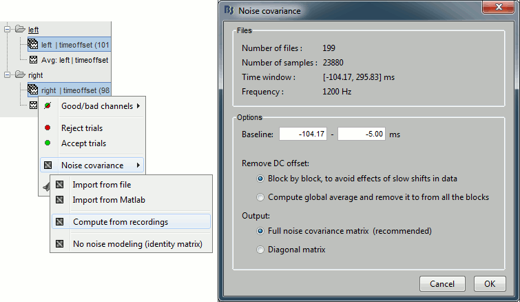
• Right-click on one of them and select: Noise covariance > Compute from recordings. Set the baseline to [-104,-5] ms, to consider as noise everything that happens before the beginning of the stimulation artifact. Leave the other options to the default values. Click on Ok.

• This operation computes the noise covariance matrix based on the baseline of all the good trials (199 files). The result is stored in a new file "Noise covariance" in the (Common files) folder.

Inverse model

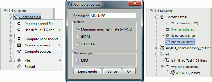
Right-click on (Common files), on the head model or on the subject node, and select "Compute sources". A shared inversion kernel is created in (Common files); a link node is now visible for each recordings file, single trials and averages. For more information about what these links mean and the operations performed to display them, please refer to the tutorial #8 "Source estimation".

Explore the sources

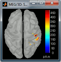
Right-click on the sources for the left average > Cortical activations > Display on cortex, or simply double click on the file. Go to the main response peak at t = 30ms, and increase the amplitude threshold to 100%. You see a strong activity around the right primary somatosensory cortex, but there are still lots of brain areas that are shown in plain red (value >= 100% maximum of the colorbar ~= 280 pA.m).

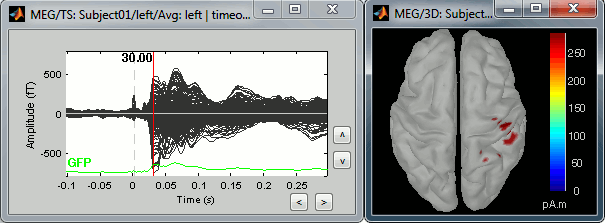
The colorbar maximum is set to an estimation of the maximum source amplitude over the time. This estimation is done by finding the time instant with the highest global field power on the sensors (green trace GFP), estimating the sources for this time only, and then taking the maximum source value at this time point. It is a very fast estimate, but not very reliable; we use it because calculating the full source matrix (all the time points x all the sources) just for finding the maximum value would be too long.

In this case, the real maximum is probably higher than what is used by default. To redefine the colorbar maximum: right-click on the 3D figure > Colormap: sources > Set colorbar max value. Set the maximum to 480 pA.m, or any other value that would lead to see just one very focal point on the brain at 30ms.

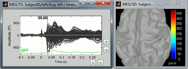
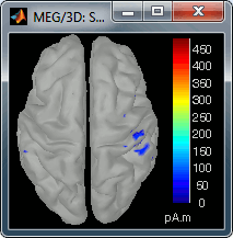
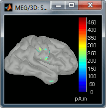
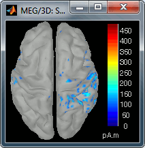
Go back to the first small peak at t=16ms, and lower the threshold to 10%. Then do what you did with at the sensor level: follow the information processing in the brain until 100ms, millisecond by millisecond, adapting the threshold and the camera position when needed:

• 16 ms (top-left): First response, primary somatosensory cortex (S1 right)

• 30 ms (top-right): S1 right

• 60 ms (bottom-left): Secondary somatosensory cortex (S2 right)

• 70 ms (bottom-right): Activity ipsilateral to the stimulus (S2 left + S2 right)

Scripting

The following script from the Brainstorm distribution reproduces the analysis presented in this tutorial page: brainstorm3/toolbox/script/tutorial_raw.m