BEst - Brain Entropy in space and time
This toolbox implements the "maximum-entropy on the mean" (MEM) technique for solving MEG, EEG and MEG/EEG source localizations. Along with the classical MEM (Amblard et al. 2004), we exploit wavelet decompositions of the data in order to target specifically oscillatory patterns (wMEM) or synchronous cortical sources (rMEM). Explanation of cMEM, rMEM, wMEM in 2-3 sentences here.
BEst, for "Brain Entropy in space and time", is the result of a collaborative work between École de Technologie Supérieure and the department of biomedical enginnering at McGill university (Montreal, Canada). The present tutorial shows how to use MEM on MEG data from
1) Simulations: 2 examples of realistic simulations of spikes
2) Inter-ictal epileptic discharges (IEDs): Average of 171 spikes
3) Median Nerve Stimulation (MNS) data: Average of 98 trials from Right hand responses
4) Sleep spindles: 5 spontaneous events
These datasets can be downloaded from here. For each dataset the anatomy and gain matrices are provided. Below we will illustrate the application of the three MEM methods on MNS dataset (BEst_tutorial_median_nerve).


See below for more info on the BEst license and the associated publications.
MEM: preliminary steps
We need one gain matrix for each recording modality considered for source localization. These matrices can be computed within Brainstorm using either, spherical or realistic (recommended) head models. See the tutorial on Head models for details. Note that unlike the other methods proposed in Brainstorm, the MEM does not require prior calculation of a noise covariance matrix. This matrix can be estimated using a physiological baseline signal that can either be part of the data to be localized or a different piece of data. We can also use empty room noise recordings if available to estimate this matrix.
- Uncompress downloaded dataset in a folder
Import the data in brainstorm by clicking: File > Load protocol > Load from folder > browse the protocol (BEst_tutorial_median_nerve)
- Go to the data view mode (second button on top of the database explorer)
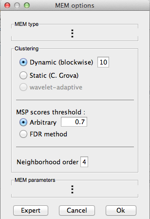
Right-click on the data average > Compute sources > BEst. Hit 'Ok' Note: The MEM option only appears in expert mode. Make sure it is toggled from the buttom at the bottom left. It is recommended that you customize the comment field so as to avoid confusion when performing multiple localizations for a given dataset.
(Figures to be included)
Select the MEM method (cMEM: temporal representation, wMEM: time-scale represenation, or rMEM: wavelet representation). Define the data time window and the baseline data while keeping other parameters at default values. Then hit 'Ok'.
(Figure to be included)
cMEM
- Selection of a specific time window may be useful for long data epochs, as cMEM is an iterative process (default: localize whole data window). Suggested time window for this dataset: 0.010s-0.030s.
- Three choices are available for baseline definition.
Default: the panel looks for a dataset called 'baseline' within the same study as the data to be localized. When not found, this option is disabled.
Within data: the baseline is a time window within the recordings.
Import: the user can import baseline data from a file using brainstorm import tools In all cases, the user can define a time window for the baseline
(Figure to be included)
Hitting 'Ok' will launch the cMEM method. At the end, a new results file appears in the database under the appropriate dataset. Simply double-click it to visualize. (Figure to be updated)

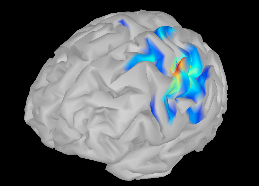
Parameters of cMEM:
- Clustering: Dynamic (Link), Stable in time (Link), MSP scores threshold (Link - Arbitrary/FDR), neighborhood order (Link), spatial smoothing (Link).
- Data definition: Time window (Link), baseline (Link).
- Expert: (Link to a page explaining the expert parameters).
wMEM
The most innovative aspect of the BEst toolbox is the application of the entropic source localization framework (MEM) on wavelet coefficients. The aim of this approach is to localize neural sources responsible for a specific activity such as oscillations or synchrony. We consider two kinds of wavelet transforms, continuous (rMEM, Zerouali et al. 2011) and discrete (wMEM, Lina et al. 2012), which make explicit the synchronous and oscillatory components, respectively.
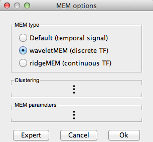
wMEM: The data is decomposed following a discrete multiresolution scheme using real Daubeachies wavelets. The time-scale plane can then be thresholded to keep only significant coefficients, up to a fraction of total signal power. The MEM then localizes the sources of each coefficient, thus yielding wavelet coefficients for each source. As we keep only significant oscillatory modes from the time-scale planes, this method efficiently targets the oscillating neural sources. Interestingly, real Daubechies wavelets have a stable inverse transform, which allows us to retrieve reald time course for each source.
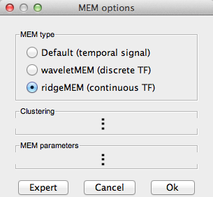
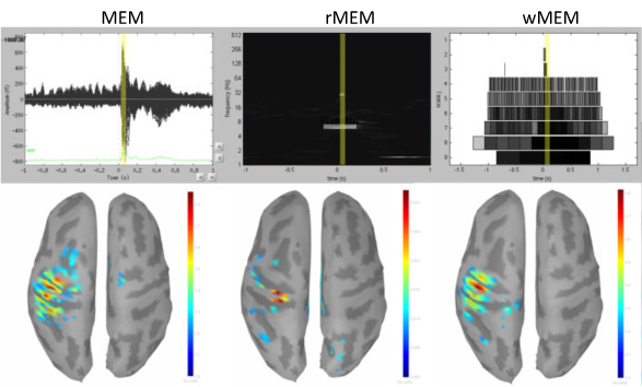
rMEM: The signal is decomposed into continuous time-frequency plane using analytic Morse wavelets. We then extract multivariate ridges from these planes, and extract the complex coefficients along the ridge lines. The sources of these complex signals are then localized using the MEM. As the ridges reflect synchronous signal components, the rMEM targets synchronous sources. The following figure illustrates the results obtained by the MEM solver and the wavelet-based MEM on Brainstorm tutorial data.
MEM fine-tuning : cortex clustering
The major prior of the MEM is that cortical activity is compartmented into discrete parcels. The activity of a given source within a patch is thus linked to the activity of its neighbors. This step is thus important for the MEM and we propose some strategies to optimize it, depending on the type of activity we target for source localization. All these approaches are data-driven and consist in two steps: sources scoring and labelling.
Sources scoring : MSP
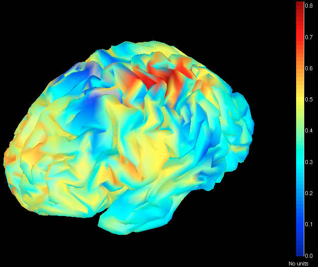
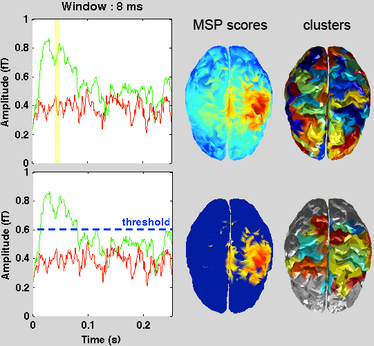
We first attribute a score to each source indicating its probability of explaining a segment of data. These scores are drawn using the multivariate source prelocalisation technique - MSP (Mattout et al. 2005, NeuroImage). The MSP proceeds by computing a signal space projector using the SVD of the normalized data segment. The leadfields of each source are then normalized and projected on that space. The L2 norm of that projection thus gives a probability-like index between 0 and 1 weighing the contribution of each source to the data (illustrated in the following figure).
Note:
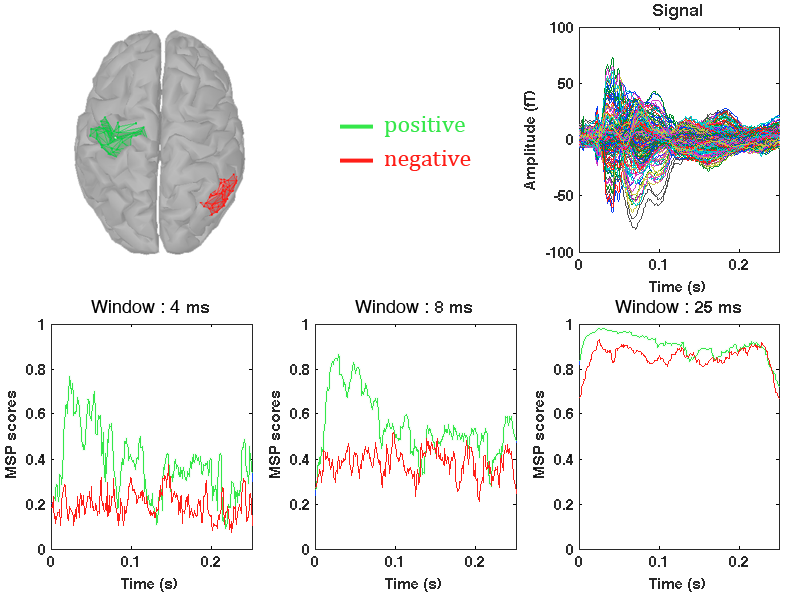
The MSP quantifies the probability for each source to explain some variability in a data segment. Implicitly, we expect the MSP scores to discriminate active regions from inactive ones in relation to the analyzed data window. In this regard, the size of the data window is an important issue. If it is too short, the variability to be explained is low and all sources will have low scores. At the opposite, if it is too large, all sources will have high MSP scores. We thus adopt two MSP strategies to obtain appropriate MSP scores distributions:
windowed MSP: (options 'blockwise' and 'wavelet-adaptive') aims at using fairly short segments of data. The size of the data segment can either be set arbitarily ('blockwise') based on empirical observations, or adapted to the temporal support of the wavelet at a given scale/frequency (only applies to wavelet-based MEM). The 'blockwise' procedure is a sliding window that computes a set of MSP scores at each time sample, thus yielding a MSP time course for each source (illsutrated in the next figure), while 'wavelet-adaptive' procedure computes a set of MSP scores for each time-frequency coefficient, thus yielding MSP time-frequency planes. These scores are then used for clustering.

canonical MSP: (option 'static') This method hypothesizes that the sources explaining the series at hand are spatially stable in time and have uncorrelated time course. It thus aims at representing cortical activity as stable parcels with evolving MSP time courses. As the scoring and the clustering are intimately related in this approach, the reader is referred to the following paper for a complete description (Chowdhury et al. 2012, NeuroImage). Briefly, we extract main components from data and build cortical patches containing sources mostly related to either one of the extracted components. The outcome of the operation is a spatially stable clustering in time but with varying MSP time courses.
Sources clustering : dynamical
The aim of this step is to group cortical sources into spatially homogenous cortical parcels based on their MSP scores. The clustering alogrithm described next is applied at each time sample thus allowing sufficient flexibility for tracking spatially moving sources while still being able to describe spatially stable sources. It proceeds as follows:
- list all vailable sources in a vector
- pick the source i with maximal MSP score
- find the neighbours of i up to the 'neighborhood order' value
- remove i and its neighbors from the list
- repeat steps 2-4 until the list is empty
Note:
It is posible to apply a threshold on the MSP scores before applying the clustering. The threshold can either be set manually or derived from a baseline using an FDR criterion (see following figure). In that case, the sources with subthreshold MSP scores are excluded from step 1 and are not part of any cluster. These sources will not be part of the MEM solution.
License
BEst is free software: you can redistribute it and/or modify it under the terms of the GNU General Public License as published by the Free Software Foundation, either version 3 of the License, or (at your option) any later version. BEst is distributed in the hope that it will be useful, but WITHOUT ANY WARRANTY; without even the implied warranty of MERCHANTABILITY or FITNESS FOR A PARTICULAR PURPOSE. See the GNU General Public License for more details. You should receive a copy of the GNU General Public License along with BEst. If not, get it here.
The references to be acknowledged are:
MEM with stable clustering. Chowdhury R, Lina JM, Kobayashi E, Grova C. MEG source localization of spatially extended generators of epileptic activity: cpmaring entropic and hierarchical bayesian approaches. PLoS One, 2012 (in revision)
wMEM. Lina JM, Chowdhury R, Lemay E, Kobayashi E, Grova C. Wavelet-based localization of oscillatory sources from magnetoencephalography data. IEEE Transactions on biomedical engineering, 2012 (Ahead of print)
rMEM. Zerouali Y, Herry C, Jemel B, Grova C. Localization of synchronous cortical neural sources. IEEE Transactions on biomedical engineering, 2011 (Ahead of print)
Additionnal references:
MSP. Mattout J, Pelegrini-Issac M, Granero L, Benali H. Multivariate source prelocalization (MSP): use of functionnaly informed basis functions for better conditioning the MEG inverse problem. NeuroImage 26: 356:373.
MEM. Amblard C, Lapalme E, Lina JM. Biomagnetic Sources Detection by Maximum Entropy on the Mean with Graphical Models, IEEE Transactions on Biomedical Engineering, 55(3): 427-442
minFunc. Schmidt M. see license