Tutorial: Import MEG recordings
Contents
Dataset description
You should already have downloaded this package if you have done correctly the previous tutorial. If it is not the case, go back to the ?previous tutorial and follow all the instructions to create the TutorialCTF protocol.
File: |
bst_tutorial_somatotopy_ctf.zip |
Acquisition system: |
CTF MEG, 151 axial gradiometers, La Salpetriere Hospital, Paris |
Protocol: |
Shuffled electrical stimulations of the thumb fingers from both hands. The idea is to get a map of the primary sensory response on the cortex |
Author: |
Data provided courtesy of Sabine Meunier |
Anatomy directory: |
- T1-MRI of the subject in CTF format (.mri) |
Datasets directory: |
- somMGYO-18av.ds: average response for the stimulation of the right thumb (one subject, 400 trials) |
Observations: |
Stimulus occurs at time 0. There's a first tiny wave occuring at about 20ms or so but it's not too clear on all fingers. So if you are to compute cortical maps, start by the 40ms peak which is also of interest and which has much better SNR. |
Import recordings
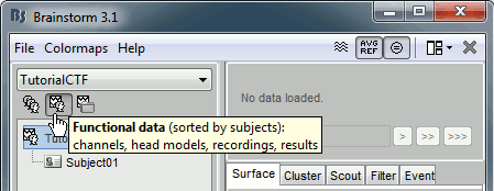
Select the TutorialCTF protocol, and go to the Functional data (sorted by subject) view of the Brainstorm database.
Right-click on Subject01, select Import MEG/EEG...
In the file format selection box, pick "MEG/EEG: CTF .ds (*.meg4;*.res4)". Go to TutorialCtf/data/ directory, select the the somMDYO-18av.ds directory and click on Open.
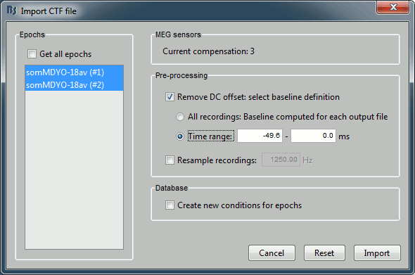
Two blocks of data are available in this file. They are referred in CTF files as Trials, even if they are the results of the averaging of trials from two different conditions.
You can select individual trials if you uncheck the "Use all trials" option.
- You can see that each block of recordings is defined for the following time range: [-49.60ms, 250.40ms]
Check the "Remove DC offset" option, together with "Base on pretrigger". For each sensor, this will compute the average value across the time (on the for the pre-trigger period, ie. where times < 0), and substract this mean to all the time values.
=> In MEG, this operation is always needed, unless it was already applied during one of the pre-processing steps.- Click on Import.
A condition was created, called after the filename. It contains three items:
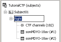
The first is the channel file: description of the positions, names, types, and various properties of the sensors that recorded the data. The value (182) means that there are 182 channels of data in the data files. They are not necessarily MEG channels, it may also includes EEG, EOG, stimulation lines, references, etc.
- The last two represent recording files
- Having the channels defined in the same file as the recordings is specific to MEG. Those systems always store all the available information at the same time. If you work with EEG, you will have to import separately the positions of the electrodes. This will be developped in an other tutorial.
Rename the condition into StimRightThumb (F2, or successive left clicks, or right-click>Rename)
Display channel file
Let's explore what you can do with the first file. Right-click on the CTF and try all the menus.
Menu: Display
The two menus in the Display menu display the same thing, but in a different way. You can add the scalp surface easily with the toolbar in the Surfaces tab, in the main window (Add a surface button).
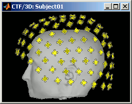
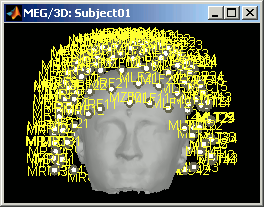
CTF axial gradiometers (only available for CTF recordings):
- All the CTF MEG sensors axial gradiometers, with one coil close to the head, and one parallel and much farther.
- This menu displays them as they will be used for the forward model computation. The small squares do not represent exactly the reality, as CTF coils are circular, but they are modelized like that.
Only the coil closest to the head is represented. The red arrows represent the orientation of the coils. Read more about ?MEG sensor types.
MEG: MEG sensors are now represented as small white dots (center of the coils close to the head), and tesselated. Red arrows still represent the orientation of the coils.
Menu: Edit channel file
Displays a table with almost all the information about the individual channels. You can use this window to view and edit the channels's properties.

The channel file describe each channel separately, with the following information:
Name : Name that was given to the channel by the acquisition device.
Type : Channel type, eg. MEG, EEG, EOG, ECG, EMG, Stim, Other, etc.
- Sometimes you will have to change the Type for some sensors; for instance if the EOG channel was saved as a regular EEG channel, you will have to change its type to prevent it from being used in the source reconstruction based on EEG.
Comment : Description of the channel.
Loc : Indicates the position in space of the sensor (x,y,z coordinates). One column per coil or per integration point; consult the pages about forward modeling theory if you want to know more about this. You should not modify these values from this interface.
Orient : Indicates the orientation in space of the sensor (x,y,z coordinates). One column per coil or per integration point.
Weight : When there are more than one coil or integration point, the Weight field indicates the multiplication factor to apply to each of these points.
Menu: File
Some other fields are present in the channel file that cannot be accessed with the Channel editor window. You can explore those other fields with the File menu, selecting View .mat files or Export to Matlab. As we saw in previous tutorial.
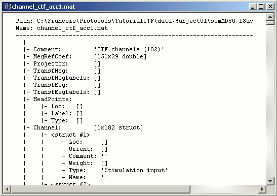
Some fields you may find there:
Comment : String that is displayed in the Brainstorm database explorer
MegRefCoef : Noise compensation matrix for CTF recordings, which is computed by the CTF softwares, based on some other sensors that are located far away from the head.
FiffInfo: Some information about coordinates systems transforms on Neuromage MEG recordings
HeadPoints: Extra head points that were digitized with a system like Polhemus Isotrak.
Menu: Align
For the moment, the registration between anatomy and sensors is based only on three points that are manually positioned (nasion and ears). This rough alignment technique is quite robust but also very unprecise, and depends only on the precision with which the people defined the fiducials, both during the data acquisition and on the MRI slices.
For this reason, it is sometimes necessary to correct the position of the sensors manually. From a scientific point of view it is not a really rigorous operation, but sometimes it is much better than using wrong automatic positions.
There are two menus: one to check the alignment head surface/sensors, and one to fix it. The Align MEG sensors menu works exactly the same way as the surface alignment tools introduced in previous tutorial (select buttons in the toolbar and right-click+move in the windows).
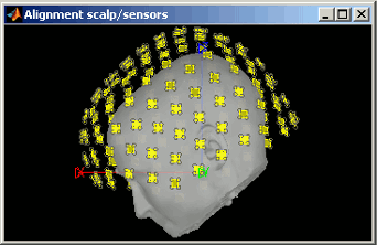
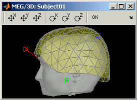
Nothing to change here, but remember to always check the registration scalp/sensors just after you import MEG or EEG recordings.
Display recordings
Just to understand what is stored in the two recording files: double-click on the first, then double-click on the second.
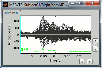
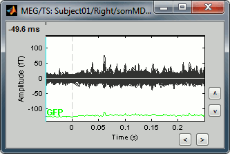
- The first one is the response to the electric stimulation averaged over 400 trials across the time (the values of each MEG sensors is represented by a black line, and they are all overlaid). Roughly, you can observe a first response peak at 23ms, and a second one at about 47ms.
- The second one is the standard deviation of the trials that were average, for each sensors and at each time.
You can rename them ERP and STD (or Error), because it makes much more sense than Somesthesie (#001) and Somesthesie (#002).
Close the windows using the Close all button on the right of the main Brainstorm toolbar. It closes all the figures at the same time and free all the memory. Try to always use this instead of closing the figures individually.

Now have a look to what is inside a recordings file: right-click on StimThumbLeft/ERP > File > View .mat file.
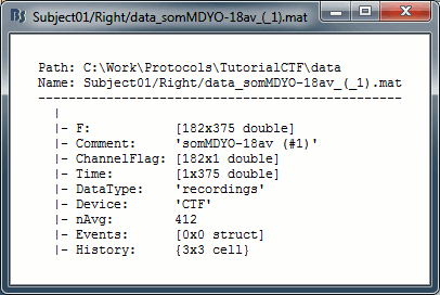
F: recordings values (nChannels x nTime)
ChannelFlag: one value per channel, 1 means good channel, -1 means bad channel (and will not be displayed or processed)
Time: Time values
Device: Name of the acquisition system used to record this file
Comment: String that is displayed in the Brainstorm database explorer to represent this file
All the recordings display tools will be discussed in the next tutorial.
Managing conditions
You have already imported the average response for the stimulation of the right thumb. Let's also import the left thumb, but proceeding in a slightly different way.
Create a new condition for your Subject01, called StimLeftThumb. To do that: right-click on Subject01 > Add condition...
Import the second file (somMGYO-18av.ds) in the StimLeftThumb condition. Rename the recordings in ERP and Std.
Switch to the Functional data (sorted by condition), by click on the third button in main Brainstorm toolbar.
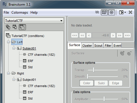
- This view is not very useful when you have one subject and two conditions. But remember this this option for later, it will be very useful when you will have 60 subjects and 12 conditions per subject in your database.
Next
Everything is now loaded in TutorialCTF protocol : subject anatomy (MRI and surfaces), recordings and channels description.
The next tutorial will present all the tools available to ?explore the recordings.