Phase-amplitude coupling
Authors: Soheila Samiee, Thomas Donoghue, Francois Tadel, Sylvain Baillet
This tutorial introduces the concept of phase-amplitude coupling (PAC) and the metrics used in Brainstorm to estimate it. These tools are illustrated first on simulated recordings. In separate tutorials, we illustrate how to use them on resting-state MEG recordings.
Contents
Introduction
Phase-amplitude coupling (PAC)
The oscillatory activity in multiple frequency bands is observed in different levels of organization from micro-scale to meso-scale and macro-scale. Studies have been shown that brain functions are achieved with simultaneous oscillations in different frequency bands [Schutter and Knyazev, 2012]. Classical studies in this field were only focused on rhythms in each of these frequency bands, and it has been reported that these rhythms are linked to perception and cognition [Cohen, 2008]. However, it is revealed that not only examining brain activity in each single frequency band, but also the relation and interaction between oscillations in different bands, can be informative in understanding brain function. Thus, this concept increasingly received interest especially in the field of cognitive neuroscience. This interaction between several oscillations is also known as cross-frequency coupling (CFC).
Two forms of recognized CFC in brain rhythms are: phase amplitude coupling (PAC), and phase-phase coupling (PPC). In the first type, which is also called nested oscillations, the phase of the lower frequency oscillation (nesting) drives the power of the coupled higher frequency oscillation (nested), that results in synchronization of amplitude envelope of faster rhythms with the phase of slower rhythms. The second form is amplitude independent phase locking between n cycles of high frequency oscillation and m cycles of low frequency one. That's why it is also called n:m phase synchrony [Palva et al., 2005].
Among these two types, phase-amplitude coupling received more interests. It has been shown that behavioral tasks can modulate the phase amplitude coupling [Voytek et al., 2010], and also it is potentially involved in sensory integration, memory process, and attentional selection [Lisman and Idiart, 1995, Lisman, 2005, Schroeder and Lakatos, 2009]. This coupling is observed in several brain regions including hippocampus, basal ganglia, and neocortex; and these observations are reported in rats, mice, sheep, and monkeys, as well as humans [Tort et al., 2010].
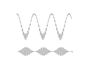
Following figure shows a schematic of phase amplitude coupling. In the top signal, we have the sum of a fast and slow oscillations, where the power of fast oscillation's envelope changes with the phase of the slower oscillation, which is a sample of PAC. The bottom signal shows only the fast oscillation and the variation in its power. As it is obvious from comparison of two signals, the fast rhythm's power is always maximum, at a certain phase of slower oscillation, this phase is called coupling phase.
Measures of cross frequency phase amplitude coupling can monitor the relationship between the activities that modulate low frequency oscillations like sensory or motor inputs, and the local cortical activities such as local computations that are correlated to amplitude of higher frequency oscillation [Canolty and Knight, 2010].
All these interesting features of this coupling resulted in proposing several methods for its measuring. Each of these methods has certain limitations and also advantages over the others, and can be used for a particular purpose; that's why no preferred standard method has been chosen for this estimation yet [Tort et al., 2010]. One of these methods, which is implemented in Brainstorm, is called Mean Vector Length (MVL), proposed by Canolty et al. (2006).
On the other hand, since phase-amplitude coupling changes over time with interinsic events and external stimuli, time-resolved estimation of this phenomena received increasing interest. Among suggested methods for estimating the dynamics of phase-amplitude coupling, tPAC [Samiee & Baillet, 2017], is implemented in Brainstorm.
These methods (MVL and tPAC) and the step by step instruction of using them are described in this section of the tutorial.
Two measures of PAC:
1. Time-resolved PAC estimation: tPAC
This approach in principle searches for the  oscillation with strongest PAC to
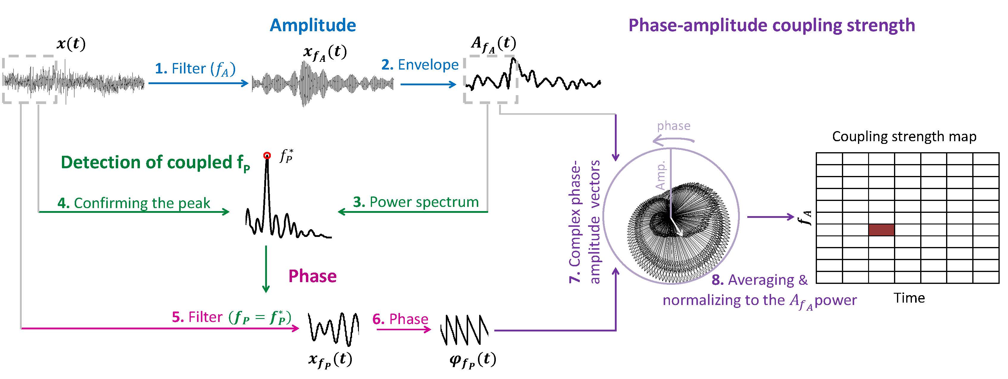
  bursts, over a time-window, which slides on the input electrophysiological data. Following figure, summarizes the steps of the algorithm (see [Samiee & Baillet, 2017] for more details).
2. Mean Vector Length (Modulation Index)
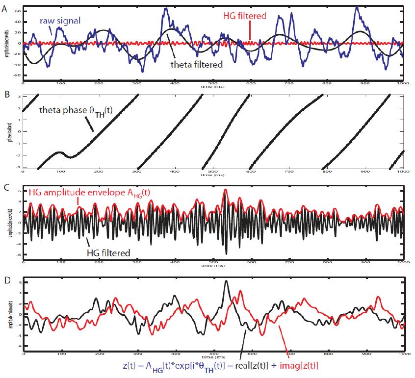
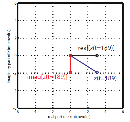
Canolty et al. (2006) pointed out that a time series defined in the complex plane by  could be used to extract a phase-amplitude coupling measure. In this formula
  is the envelope of fast oscillation, and
  is the phase of slow oscillation.
Therefore, after filtering in fast and slow oscillation, and extracting the phase of slow, and the amplitude of fast rhythm; each instantaneous fast oscillation amplitude component in time is represented by the length of the complex vector, whereas the slow oscillation phase of the same time point is represented by the vector angle (see following figure).
At the absence of phase-amplitude coupling, the plot of the  time series in the complex plane is characterized by a roughly uniform circular density of vector points, symmetric around zero, because the
  values (averaged over cycles of slow oscillation) are approximately the same for all phases. If there is modulation of the
  amplitude by the
  phase, the
  would be higher at certain phases than others. This higher amplitude for certain angles will lead to a “bump” in the polar plot of the
  , leading to loss of symmetry around zero. This loss of symmetry can be inferred by measuring the length of the vector obtained from the mean over all points in the complex plane. It is thus assumed that a symmetric distribution as it occurs during lack of coupling leads to a small mean vector length (because the points in the different phases would cancel each other), whereas the existence of coupling leads to a larger mean vector length [Tort et al. 2010]. For more detail read [Canolty et al, 2006].
References
Canolty RT, Edwards E, Dalal SS, Soltani M, Nagarajan SS, Kirsch HE, Berger MS, Barbaro NM, Knight RT (2006). High gamma power is phase-locked to theta oscillations in human neocortex, Science, 313(5793), 1626-1628.
Canolty RT, Knight RT (2010). The functional role of cross-frequency coupling. Trends in cognitive sciences, 14(11), 506-515
Cohen MX (2008). Assessing transient cross-frequency coupling in EEG data. Journal of neuroscience methods, 168(2), 494-499.
Palva JM, Palva S, Kaila K (2005). Phase synchrony among neuronal oscillations in the human cortex. The Journal of Neuroscience, 25(15), 3962-3972.
Samiee, Soheila, and Sylvain Baillet (2017). Time-resolved phase-amplitude coupling in neural oscillations. NeuroImage, 59, 270-279.Schutter DJ, Knyazev GG(2012). Cross-frequency coupling of brain oscillations in studying motivation and emotion. Motivation and emotion, 36(1), 46-54.
Tort AB, Komorowski R, Eichenbaum H, Kopell N (2010). Measuring phase-amplitude coupling between neuronal oscillations of different frequencies. Journal of neurophysiology, 104(2), 1195-1210.
Voytek B, Canolty RT, Shestyuk A, Crone NE, Parvizi J, Knight RT (2010). Shifts in gamma phase–amplitude coupling frequency from theta to alpha over posterior cortex during visual tasks.Frontiers in human neuroscience, 4.
Simulate signals
For PAC analysis you can use your own data, or generate a synthesized data containing cross-frequency phase-amplitude coupling, with your preferred parameters. Here we explain how to produce simulated data. The model used for data generation is a simple method introduced in [Tort et al. 2010]. In this section, we generate a dataset of synthesized signal and analyze it with available phase-amplitude coupling estimation tool in brainstorm.
Select the menu File > Create new protocol > "TutorialPac" and select the options:
"Yes, use protocol's default anatomy",
"No, use one channel file per condition".
Right-click on the TutorialPac folder > New subject > Subject01
In the Process1 tab, leave the file list empty and click on the button [Run]
Select the process "Simulate > Simulate PAC signals".
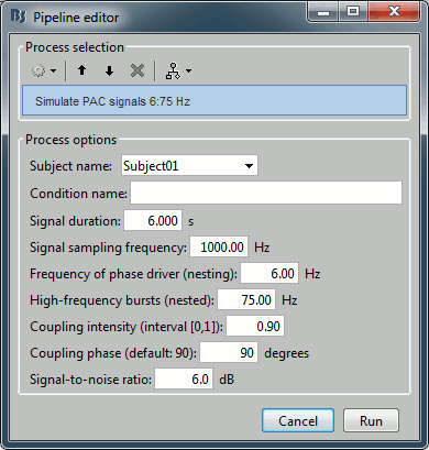
Set all the parameters as follows:
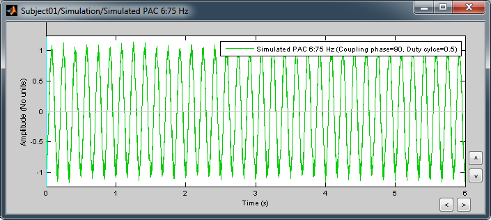
After running the process, you'll get a synthesized data file:
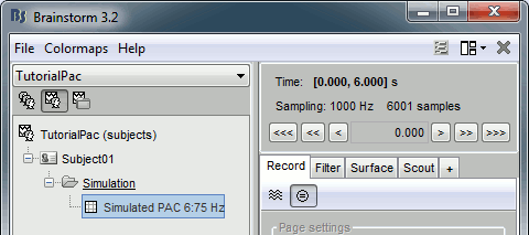
Double-click on it to display the generated signal:
Process options
Subject name: Specify in which subject the simulated file is saved.
Condition name: Specify the folder in which the file is saved (default: "Simulation").
Signal sampling frequency: Sampling frequency of the simulated signal in Hz.
Nested and nesting frequency: Definition of the phase-amplitude coupling.
Coupling intensity: Value between 0 and 1 which determines how coupled the two oscillations are.
Coupling phase: Phase of slow oscillation (phase driver) where we have the maximum envelope of fast oscillation (high frequency bursts). For example, if
 =90 degree, the maximum coupling happens in the peaks of slow oscillation.
 Signal-to-noise ratio: Determines the power of the noise that will be added to the pure coupled oscillations. This noise composed of two parts: a component with 1/f spectrum which simulate the background brains activity, and a white noise which represents the noise of data recording.
PAC estimation with MVL
Input data
You can use your own data set, or the signal that is generated with brainstorm simulator. Here we used the simulated signal that is generated with the steps explained in the previous section.
PAC estimation
To extract the phase-amplitude coupling from this signal:
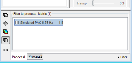
Drag the simulated file to the Process1 tab:
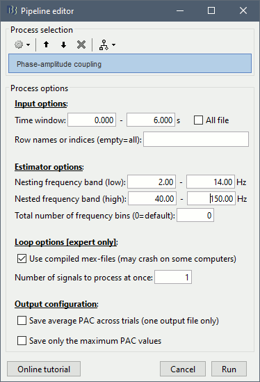
Select the process "Frequency > Phase-amplitude coupling"
Set the parameters as follows:
The PAC map calculated from your simulated signal is saved in a new file. Double click on it.
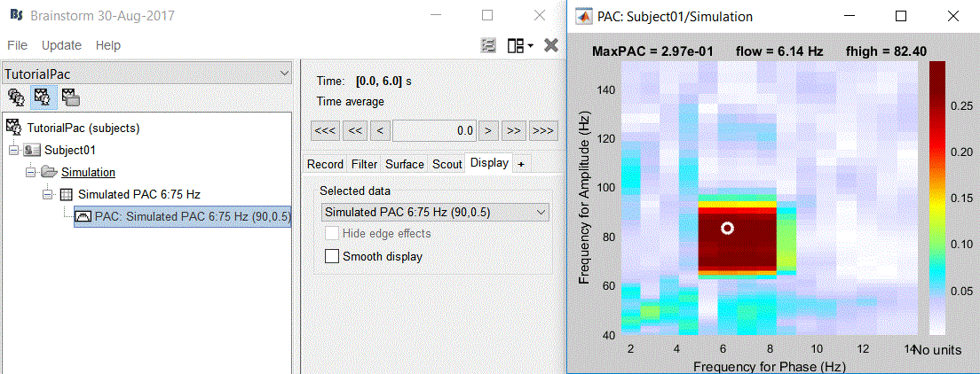
- This coupling map, also known as comodulogram, shows the cross-frequency coupling in frequency domain. The pseudo color of the map indicates the level of coupling between each pair of low and high frequencies. The abscissa represents the frequencies analyzed as phase frequency, while the frequencies for amplitude are represented in the ordinate axis.
Here, in this example, there is a bump around 6-8 Hz for the phase and 70-85 Hz for the amplitude, which contains the pair that we initially used for synthesizing the data.The parameters of the point with maximum coupling intensity in the map will be shown in the title of the figure. These parameters are the maximum pac level, and the corresponding
 and
and  , which are 0.3, 6.14 Hz, and 80.18, respectively Hz in this case.
Process options
Input options:
Time window: The time segment of the input file to be analyzed for PAC.
Row names or indices: The name of channels to be processed in the case of input files containing multiple signals. If empty, it will process all the signals in the file.
Estimator options:
Nesting frequency band (low): Frequencies to consider for slow oscillation (frequency for phase).
- Can be a wide exploratory range (2-30Hz) or a smaller specific range (theta: 4-8Hz)
Nested frequency band (high): Freq to consider for high freq bursts (frequency for amplitude)
- Can be a wide exploratory range (40-250 Hz) or a smaller specific range (low gamma: 40-80Hz)
- Note: Nested frequencies can only be as high as your sampling rate has the resolution to yield
Total number of frequency bins: Set the total number of frequency bins estimated, for both the nesting and nested frequency bands.
Loop options: Should be left at default options unless you know how to use them.
Use mex-files: Compiled mex-files are available for running this process and contribute to speeding up the computation time.
Number of signals to process at once: The file that is given to the function is processed in blocks of signals, and this option signifies how many signals are in each block. Increasing this value can make the process a bit faster but requires a large amounts of memory.
Output options:
Save average PAC across trials: If this box is selected and multiple files have been given to the process, then the process will save the average PAC across all trials in a new file.
Be careful with this option: although it is offered, averaging over frequencies (such as is required to do this) can be problematic and results from this option should be interpreted carefully.Save only the maximum PAC value: If this option is selected then only the frequency pair with the maximum PAC coupling is saved for each signal in input (maxPAC), instead of the full PAC comodulogram. The default option is to save all the PAC values for each and every frequency pairing for each and every signal.
- Saving the full PAC maps entails saving a matrix of [Nsignals x 1 x Nfa x Nfp], this will very quickly create very large files. Check this option if the files generated are too large to display, save or process on your computer.
- The maxPAC is not a very stable estimator of the most significant frequency pairing in the comodulograms, so it can be usefull to save all the values for a visual inspection of the full PAC maps.
File contents
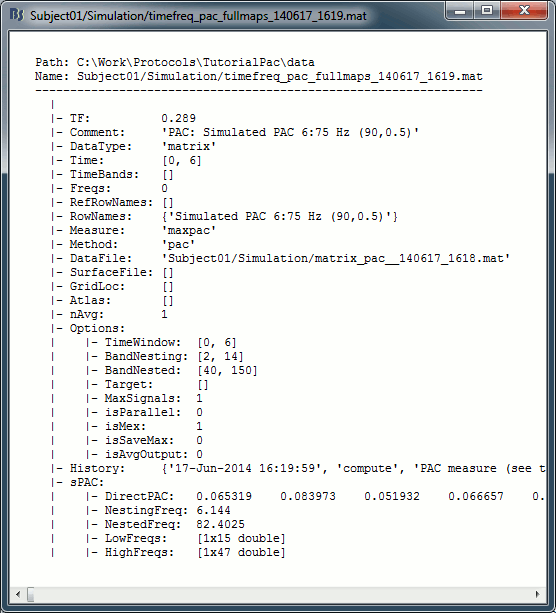
The files saved by this process have the same structure as the time-frequency files, with an additional "sPAC" field. To review its contents, right-click on the PAC file > File > View file contents.
Some of the relevent fields in the maxPAC files:
TF: [Nsignals x 1 x 1], Coupling strength of the maximally coupled frequency pairing (maxPAC)
Options: All the parameters that were given to the process
sPAC: All the additional information related to the output of the PAC function
DirectPAC: [Nsignals x Ntime x Nlow x Nhigh], PAC values for all the frequency pairings
NestingFreq: [Nsignals x 1], Low frequency at the maxPAC
NestedFreq: [Nsignals x 1], High frequency at the maxPAC
LowFreqs: [Nlow x 1], List of low frequencies used for the DirectPAC matrix
HighFreqs: [Nhigh x 1], List of high frequencies used for the DirectPAC matrix
Recommendations
PAC estimation using the MVL algorithm
In order to have a reliable result from this method it is required to use a signal which length is at least ten cycles of the slowest oscillation in your low oscillation band.
Considering this point is more important in analysis of real databases, where the noise level (and/or background brain activity) can be higher than synthesized data, and the coupling intensity can be low. Thus, if you want to examine the coupling for slow oscillations in [2, 14] Hz, it would be better to use a signal with minimum length of 10 cycles of the slowest oscillation, which would be 10 x 0.5 = 5 S.
Time-resolved PAC estimation with tPAC
Input data
For tPAC estimation you can use your own data set or simulated data. For illustration here, we simulated three time series with phase-amplitude coupling using brainstorm tool and combine them. The script to reproduce such signal can be found here. The resulting time series looks like:

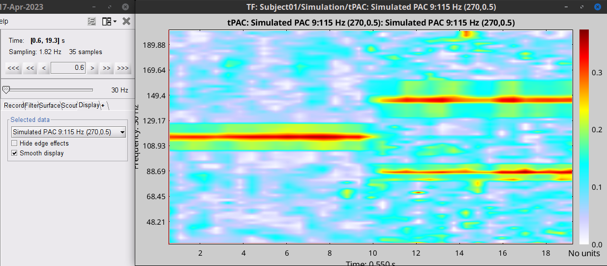
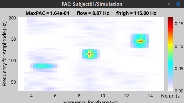
During the first half of the signal (10 s duration), the phase of slow oscillation at 9 Hz is coupled to the amplitude of a faster rhythm at 115 Hz. In the second half, the first coupling mode is terminated and the average of two other simultaneous modes appears. These modes are  = 13 Hz,
  = 145 Hz, and
  =5 Hz,
  =87 Hz, respectively. The signal-to-noise ratio is set to 6 dB, and the preferred coupling phase in the three modes are 270, 0, and 180°, respectively. The coupling strength is kept constance and identical in all modes.
Time-resolved PAC
To extract the phase-amplitude coupling from this signal:
- Drag the simulated file (or real data) to the Process1 tab:
Select the process "Frequency > Time-resolved Phase-amplitude coupling > tPAC"
Set the parameters as follows (these parameters are explained later in the text):
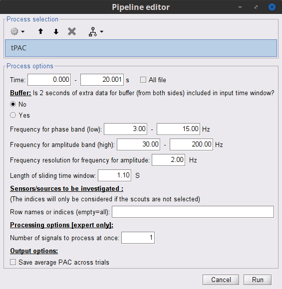
- The PAC map calculated from your simulated signal is saved in a new file. Double click on it.
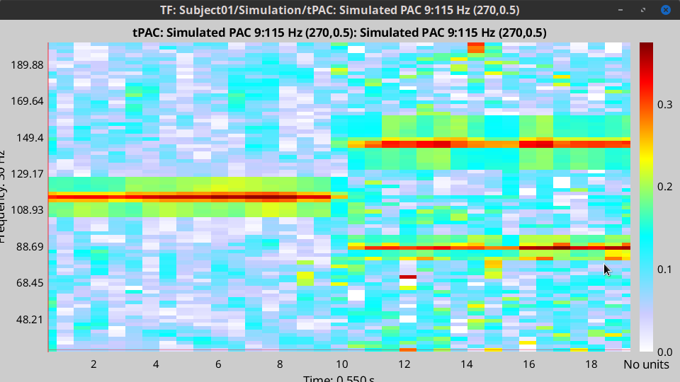
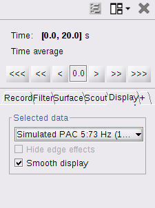
- You can smooth the map with activating the smooth display button:
This coupling map, shows the cross-frequency coupling in time-
 domain. The pseudo color of the map indicates the level of coupling in each time-interval for each
  .
. Here in this example there is one mode around
 Hz in the first 10 seconds, and two other modes appear in the second half of the signal on around 85 Hz, and 145 Hz, which reflect the oscillations that we initially used for synthesizing the data.
 This map is a 2D projection of three dimensional phase-amplitude coupling (time,
 , and
, and  ). For investigating other dimensions you can project it on other planes of
  and time-
 using available tools in brainstorm (see below).
Process options
Input options:
Time window: The time segment of the input file to be analyzed for time-resolved PAC.
Row names or indices: The name of channels to be processed in the case of input files containing multiple signals. If empty, it will process all the signals in the file.
Buffer: Is 2 seconds of extra data included in ...
No: zero padding will be used for edge effect reduction
yes: 2 seconds of data (from both sides) will be used as buffer for reducing edge effect in filtering (recommended, especially if the input data is long the margins are not super important)
Estimator options:
Frequency for phase band (low): Frequencies to consider for slow oscillation. It can be a wide exploratory range (2-30Hz) or a smaller specific range (theta: 4-8Hz)
Frequency for amplitude band (high): Frequencies to consider for high frequency bursts. It can be a wide exploratory range (40-250 Hz) or a smaller specific range (low gamma: 40-80Hz).
- Note: The lower bound of the frequency-for-amplitude band must be at least twice the upper bound of the frequency-for-phase band.
Frequency resolution for frequency for amplitude: This value indicates the bandwidth of the subbands in which the band
 will be divided.
 Length of sliding time-window: Should at least include one full cycle of minimum
 of interest (entered above).
 - Decreasing its length will improve temporal resolution, but decrease resolution for frequency for phase, and will also increase the processing time
If you have a event-related design for your study with more than 100 trials, and need very high temporal resolution (e.g. below 5 ms), you can use event-related PAC (ERPAC) algorithm (not implemented in brainstorm).
Number of signals to process at once: The file that is given to the function is processed in blocks of signals, and this option indicates how many signals will be processed simultaneously. Increasing this value can make the process a bit faster but requires a large amounts of memory.
Output options:
Save average PAC across trials: If this checkbox is selected and multiple files have been given to the process, then the process will save the average PAC across all trials in a new file.
Be careful with this option: although it is offered, averaging over frequencies (such as is required to do this) can be problematic and results from this option should be interpreted carefully.
File contents
The files saved by this process have the same structure as the time-frequency files, with an additional "sPAC" field. To review its contents, right-click on the PAC file > File > View file contents.
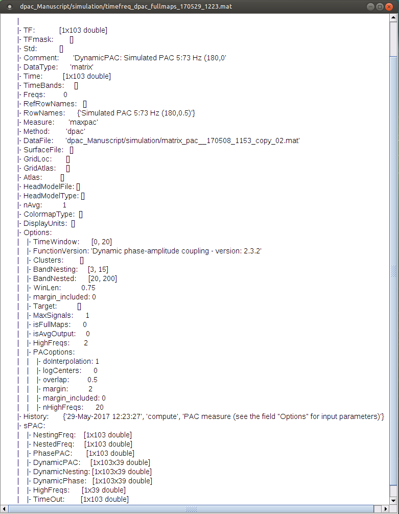
Note: Preferred phase of coupling extracted for each pair of  -
- is saved under sPAC.DynamicPhase. It can be exported to matlab and visualized there.
Comodulogram of time-resolved PAC:
To extract the comodulogram from the time-resolved PAC:
- Drag the time-resolved PAC file/files to the Process1 tab:
Note: if you have more than one time-resolved PAC file (e.g. from different trials), it is better to extract on comodulogram from all of them together to increase the SNR (considering the sparse nature of PAC in the three-dimensional time-
 -
- plane
plane
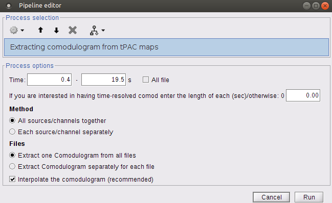
Select the process "Frequency > Time-resolved Phase-amplitude coupling > Extracting comodulogram from tPAC maps"
- Set the parameters as follows (these parameters are explained later in the text):
- The PAC map calculated from your simulated signal is saved in a new file. Double click on it.
This coupling map, shows the cross-frequency coupling in
 -
- domain. The pseudo color of the map indicates the level of coupling for each pair of frequencies.
 Here in this example there is one mode arouond
 Hz in the first 10 seconds, and two other modes apear in the second half of the signal on around 85 Hz, and 145 Hz, which reflect the oscillations that we initially used for synthesizing the data.
Process Options
Input options:
Time window: The time segment of the input file to be analyzed for extracting comodulogram.
Time-resolved Comodulogram:
- Input should be in second
- It is recommended to leave it as default: 0 -- extract one comodulogram from the total file
- Not recommended: If you would like to see the movie of time resolved comodulogram (in current set up of the brainstorm it can only be played in matlab and only once when it is computed), enter the window length to estimate several comodulograms each with that length from input tPAC map. -- You can zoom in/out in played movie in matlab.
Method:
- Method for estimating comodulogram. The method will be the same for both options if you have only one input (like this example with simulated data.
All sources/channels together: select this option if all sources belong to the same scout, or you do not expect different responses from them. (This will increase the SNR for comodulogram estimation, and make it more accurate and less noisy)
Each source/channel separately:
Time-resolved PAC in time -  domain
...
Further analysis of PAC files
All functions for further analysis of PAC files (e.g., deriving the average of PAC maps, producing comodulograms, running a z-score transform with respect to baseline levels or surrogate data, etc. ) are available as processed located in Frequency > Time-resolved Phase-amplitude coupling.

Note: Basic functions for averaging or running statistics are not yet avalaible with Brainstorm [working on it...]. Yet, PAC output files are stored as Matlab files and contents can be readily processed with custom scripts of your own.
Yet, surrogate analysis is only available for single band tPAC maps, and can be accessed here: 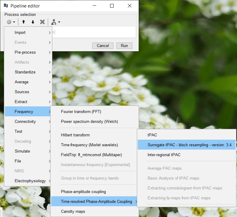
Further, tPAC traces can be z-scored with respect to surrogate data using the Process2 tab.
Practical suggestions for PAC analysis
How to best get started with PAC analysis? How do you decide about setting parameters? Here, we provide basic recommendations that we hope can be helpful:
General suggestions
- First, decide which frequency bands of interest for the frequency for phase (fP) and the frequency for amplitude (fA). These bands are usually hypothesized from the neurophysiological mechanisms you wish to study. If you have no previous clue from previous literature etc. you may want to start with visualizing the power spectrum density (PSD) of the empirical signals. It is recommended to define the fP band around a visible peak of the PSD [Aru et al. 2015], which indicates strong rhythmic signalling.
If you are not sure about the fA band, which can be elusive in PSD plots, you may first define it as a relatively wide frequency band. The resulting comodulogram output (i.e. a map with
 and
and  in horizontal and vertical axis, respectively, and a pseudo color illustrating the intensity of the coupling between each pair of frequencies) may indicate the restricted range of fA where PAC is more strongly expressed, for further single-band PAC analysis (see above).
 The intensity of PAC coupling is often stronger for slower fP oscillations. This is due in part to greater signal strengths at lower frequency in electrophysiological data (think 1/f power decrease). We therefore recommend that you subdivide a possibly wide frequency band of interest for
 in to 2 or 3 narrower bands. This approach may also provide insight about possibly co-existing modes of PAC (i.e. having several [fP,fA] pairs coupled with PAC). It also prevents PAC modes at slower fP masking other modes. For example, if you want to investigate coupling between slow rhythms in from delta to beta bands (2-30 Hz) for
  and gamma oscillations for
  , we recommend you run PAC twice: first with delta to theta (2-8 Hz) for
  , then again with alpha to gamma (8-30 Hz).
Time-resolved analysis
For time-resolved analysis, if you are not sure about the exact frequencies that you want to focus on, one practical pipeline is to extract comodulogram with a relatively wide band (based on your initial hypothesis), and then find the main mode of coupling from the comodulogram. In the next step, focus on that particular mode of coupling to evaluate dynamical changes in coupling intensity (or preferred phase of coupling) with a single band analysis (single band option does not provide comodulogram but reflect a trace of dynamical changes in coupling parameters). With this strategy the temporal resolution will be optimized for the main mode of coupling, and also the computational load for intensive analysis (and checking significance of outcomes) will be much lower than looking at the whole interval.
Following steps provide more details:
- Start with comodulogram and find the main mode (or modes) of coupling based on comodulogram.
To decide about length of sliding time window in this step, you can start with two cycles of the slowest oscillation in the band of interest for
 . For example, if you are interested in investigating potential PAC between theta to alpha oscillations (4-12 Hz) for
  and gamma rhythms for
  , a conservative short sliding time window can be set to two cycles of 4 Hz (i.e.
  . Certainly, if you have long inputs increasing the length of the window would improve the SNR.
The only point that you should keep in mind is that, tPAC do sparse estimation of PAC in a 3D space of fP, fA and time; therefore, you need enough number of points in time dimension to be able to retrieve a reasonable projection of it on fp - fA plain (called comodulogram). Hence, the maximum length of the window can be selected based on the input length. For example, in the case where your data is around 5 minutes long, if you set the window length to 20 s, considering the 50% overlap of windows you will end up with 5 * 60s / 10s = 30 points along time dimension (which is used in averaging for comodulogram extraction). It is not recommended to go below a certain number (e.g 30).
For extracting comodulogram you can also use none-time-resolved option (e.g. MVL) which use the whole time window and does not divide it into smaller chunks. It should be noted that in one experiment we observed higher resolution from comodulogram extracted using time-resolved method compared to a traditional option (see Fig. 5 in [Samiee & Baillet 2017]: https://www.sciencedirect.com/science/article/pii/S1053811917306195#fig5). The reason behind this improvement could be similar to the improvement in power spectral density estimation using Welch approach compared to original Bartlett's method.
- If you can find an obvious mode of coupling in the comodulogram, it would be better to investigate that mode of coupling using single band analysis for all regions of interest and time intevals (rather than maxPAC value extracted from comodulogram).
- If there is no obvious mode of coupling in averaged comodulogram, it is not recommended to go further in analysis. It would be better to take a more close look at modes availble in each single recording, and consistancy of preferred phase of coupling in time and in different trials/subjects.
If you observe a blub in comodulogram which looks like a vertical line, you need to further investigate your data to make sure this observed coupling is not a pseudo coupling coming from sharp event artifacts (e.g. spikes in LFP) or asymmetric oscillations (e.g. oscillations with saw tooth waveform shape). See [Cole & Voytek 2017; Aru et al. 2015] for more details.
A quick summary of the most important practical points in PAC analysis
1. Temporal resolution and minimum 
Temporal resolution, and frequency resolution are complementary to each other. The minimum
 that can be evaluated is equal 1/sliding time window, which means we need at least one cycle of minimum
  of interest in each sliding time window. For example if your
  band of interest is [4 - 8 Hz], minimum window length is 1/4 = 0.25 s.
2. Suggestion for deciding about initial  band
band
If you do not have any priori hypothesis about which frequency band could be involved in the task as
 , you can look at the power spectrum of the original signal. One of the requirements for having a PAC is a clear peak in that power spectrum around
  . For example if there is a peak around theta oscillations you can define your band of interest as 4 - 8 Hz.
3. Coupling strength for the main coupled pair
After detection of the best coupled
 and
and  , you can run tPAC with single
  band option only around that pair of interest. The window length can also get decreased to include at least two cycles of
  (May increase the temporal resolution compared to initial investigation because
  could be higher than the minimum
  in our band of interest). The output will be a time-series of PAC strength for that band of interest.
