Artifact cleaning with SSP

It is common to have portions of recordings contaminated by events coming from the subject (eye blinks, movements, heartbeats, teeth clenching, implanted stimulators...) or from the environment (stimulation equipment, elevators, cars, trains, building vibrations...). Some of them are well defined, reproducible and can be removed efficiently using Signal Space Projections (SSP). The purpose of this tutorial is to introduce this technique to correct for the cardiac and ocular artifacts.

For this tutorial, we are going to use the protocol created in the previous tutorial ?Review continuous recordings and edit markers. If you have not followed this tutorial yet, please do it now.

Signal Space Projection

The Signal-Space Projection (SSP) is one approach to rejection of external disturbances. Here is a short description of the method by Matti Hämäläinen, from the MNE 2.7 reference manual, section 4.16.

Unlike many other noise-cancellation approaches, SSP does not require additional reference sensors to record the disturbance fields. Instead, SSP relies on the fact that the magnetic field distributions generated by the sources in the brain have spatial distributions sufficiently different from those generated by external noise sources. Furthermore, it is implicitly assumed that the linear space spanned by the significant external noise patterns has a low dimension.

Without loss of generality we can always decompose any n-channel measurement b(t) into its signal and noise components as:

• b(t) = b_s(t) + b_n(t)

Further, if we know that b_n(t) is well characterized by a few field patterns b₁...b_m, we can express the disturbance as

• b_n(t) = Uc_n(t) + e(t) ,

where the columns of U constitute an orthonormal basis for b₁...b_m, c_n(t) is an m-component column vector, and the error term e(t) is small and does not exhibit any consistent spatial distributions over time, i.e., C_e = E{ee^T} = I. Subsequently, we will call the column space of U the noise subspace. The basic idea of SSP is that we can actually find a small basis set b₁...b_m such that the conditions described above are satisfied. We can now construct the orthogonal complement operator

• P_⊥ = I - UU^T

and apply it to b(t) yielding

• b(t) ≈ P_⊥b_s(t) ,

since P_⊥b_n(t) = P_⊥Uc_n(t) ≈ 0. The projection operator P_⊥ is called the signal-space projection operator and generally provides considerable rejection of noise, suppressing external disturbances by a factor of 10 or more. The effectiveness of SSP depends on two factors:

1. The basis set b₁...b_m should be able to characterize the disturbance field patterns completely and

2. The angles between the noise subspace space spanned by b₁...b_m and the signal vectors b_s(t) should be as close to π/2 as possible.

If the first requirement is not satisfied, some noise will leak through because P_⊥b_n(t) ≠ 0. If the any of the brain signal vectors b_s(t) is close to the noise subspace not only the noise but also the signal will be attenuated by the application of P_⊥ and, consequently, there might by little gain in signal-to-noise ratio.

Since the signal-space projection modifies the signal vectors originating in the brain, it is necessary to apply the projection to the forward solution in the course of inverse computations.

For more information on the SSP method, please consult the following publications:

• C. D. Tesche, M. A. Uusitalo, R. J. Ilmoniemi, M. Huotilainen, M. Kajola, and O. Salonen, "Signal-space projections of MEG data characterize both distributed and well-localized neuronal sources," Electroencephalogr Clin Neurophysiol, vol. 95, pp. 189-200, 1995.
• M. A. Uusitalo and R. J. Ilmoniemi, "Signal-space projection method for separating MEG or EEG into components," Med Biol Eng Comput, vol. 35, pp. 135-40, 1997.

Identify the artifact

The first step is to identify several repetitions of the artifact (the vectors b₁...b_m). We need to set markers in the recordings that indicate when the events that we want to correct for occur. To help with this task, it is recommended to always record with bipolar electrodes the activity of the eyes (electro-oculogram or EOG), the heart (electro-cardiogram or ECG), and possibly other sources of muscular contaminations (electromyogramor EMG). In this example, we are going to use the ECG and EOG traces to mark the cardiac activity and the eye blinks. Two methods can be used, manual or automatic.

EOG/ECG channels

• Select the protocol TutorialRaw created in the previous tutorial, and select the "Functional data" view (second button in the toolbar on top of the database explorer).

• Double-click on the continuous recordings ("Link to raw file") to open the MEG recordings.

• Set the length of the reviewed time window to 3 seconds (in the Event tab, text box "Duration")

• Right-click on the continuous recordings again > Misc > Display time series.
  
  

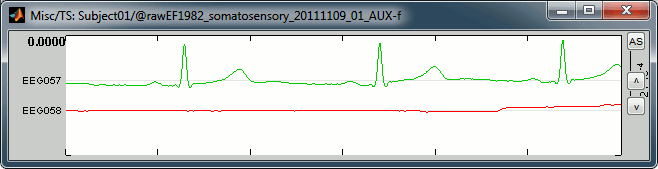
• In this file the channel type "Misc" groups the two channels EEG057 (ECG, in green) and EEG058 (EOG, in red). This configuration depends on the acqusition setup, and can be redefined afterwards in Brainstorm (right-click on the channel file > Edit channel file, and then change manually the string in the column Type for any channel).

• Use the shortcuts introduced in the previous tutorial to adjust the vertical scale of this display: Shift+mouse wheel, +/- keys, or the buttons on the right side of the figure.

• Then go further in time to see what is happening on those channels over the time: use the ">>>" buttons, or the associated shortcuts (read the tooltips of the button)

• ECG: On the green trace, you can recognize the very typical shape of the electric activity of the heart (P, QRS and T waves). This is a very good example, the signal is not always that clean.

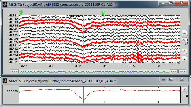
• EOG: On the red trace, there is not much happening for most of the recordings except for a few bumps, typical of eye blinks, eg. at 33.590s. This subject is sitting very still and is not blinking much. We can expect MEG recordings of a very good quality.

• You can observe the contamination from a blink on the left-frontal sensors: move to 33.590s (you can use the text boxes in the time panel, the event tab, or the scrollbar in the figure), and select a subset of sensors (Shift+B, or right-click on the figure > Display setup > CTF LF)
  
  

Manual marking

Create a new category of markers "blink_manual", using the menu Events > Add group. Select this new group. Review the file, and mark the peaks you observe on the EOG trace, using the Ctrl+E keyboard shortcut. Do that for a few eye blinks.

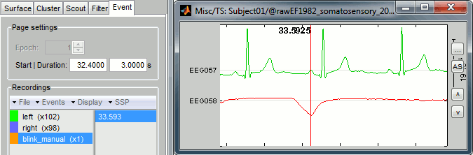
You could repeat the same operation for all the blinks, then for all the ECG peaks and jump to the next chapter of the tutorial and compute the SSP. It would be uselessly time consuming, as there is a process that does it for you automatically. However, it is good to remember how to do it manually because you may face some cases where you don't have clean ECG/EOG, or if you want to correct for another type of artifact.

Automatic detection: ECG

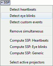
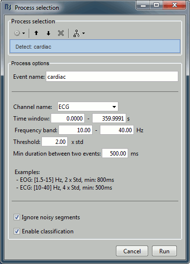
In the event tab, select the menu: SSP > Detect heartbeats. It opens automatically the pipeline editor, with the process "Detect heartbeats" selected:

• Channel name: Name of the channel that is used to perform the detection. Select or type "EEG057" as it is the name of the ECG channel

• Time window: Time range that the algorithm should scan for the selected artifact. Leave the default values to process the entire file. Ignore the small rounding errors that lead to displaying a very small negative value instead of "0".

• Event name: Name of the event group that is created for saving all the detected events. Leave the default "cardiac".

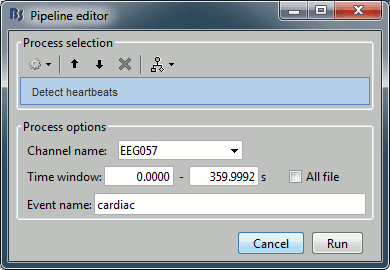
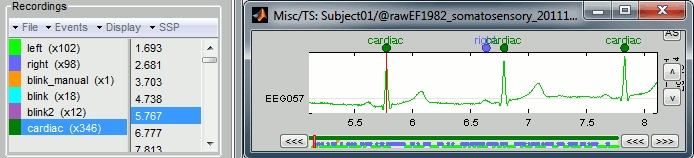
Click on Run. After the process stops, you can see a new event category "cardiac" in the events tab, with 346 occurrences. You can check a few of them, to make sure that the "cardiac" markers really indicate the ECG peaks, and that there are not too many peaks that are skipped. In the event tab, click on the "cardiac" event category, then on a time occurrence to jump to it in the MEG and Misc time series figures.

Automatic detection: EOG

Now do the same thing for the eye blinks. In the event tab, select the menu "SSP > Detect eye blinks". Configure the process to use the channel EEG058 (name of the EOG channel), and leave the other options to the default values.

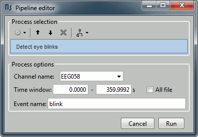
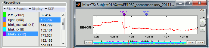
The result of this process is slightly different from the heartbeat detection: it created two event groups instead of one, "blink" and "blink2". Indeed, this algorithm not only detects specific events in a signal, it also classifies them by shape. If you go through all the events that were detected in the two categories, you would see that the "blink" are all round bumps, typical of the eye blinks, while the "blink2" are ramps followed by sharp drops, a shape that indicates an eye saccade.

Automatic detection: Custom

Those two previous processes are shortcuts for a generic process "Detect custom events". We are not going to use it here, but it is interesting to introduce it to understand how the blinks and heartbeats detection work. The logic is the following:

• The channel to analyze is read from the continuous file, for a given time window.

• Frequency band: The signal is filtered in a frequency band where the artifact is easy to detect. For EOG: 1.5-15Hz ; for ECG: 10-40Hz.

• Threshold: An event of interest is detected if the absolute value of the filtered signal value goes over a given number of times the standard deviation. For EOG: 2xStd, for ECG: 4xStd

• Minimum duration between two events: If the filtered signal crosses the threshold several times in relation with the same artifact (like it would be the case for muscular activity recordings on an EMG channel), we don't want to trigger several events but just one at the beginning of the activity. This parameter prevents the algorithm from detecting other events immediatly after a successful detection.
  For the ECG, this value is set to 500ms, because it is very unlikely that the heart rate of the subject goes over 120 beats per minute.

• Ignore the noisy segments: If this option is selected, the detection is not performed on the segments that are much noisier than the rest of the recordings.

• Enable classification: If this option is selected, the events are classified by shape, based on correlation measure. In the end, only the categories that have more than 5 occurrences are kept, all the other successful detections are ignored.

Calculate the projector

Methodology

We have now 346 examples of heartbeats, 18 examples of blinks, and 12 examples of saccades. Those are sufficient numbers of repetitions to calculate reliable signal-space projections. The logic of the computation is the following:

1. Take a small time window around each marker to capture the full effect of the artifact, plus some clean brain signals before and after.
2. Filter the MEG or EEG signals in a frequency band of interest, in which the artifact is the most visible.

3. Concatenate all those time blocks into a big matrix A = [b₁, ..., b_m]

4. Compute the eigenvalue decomposition of this matrix A: [U,S,V] = svd(A, 'econ')

5. The eigenvectors Ui with the highest eigenvalues Si are an orthonormal basis of the artifact subspace that we want to subtract from the recordings. The software selects by default the vectors with eighvalues above a certain threshold: Si > 12% * sum(Si)
   Then it is possible to redefine interactively the selected components.

6. Calculate the projection operator: P_⊥ = I - UU^T

7. Apply this projection on the MEG or EEG recordings F: F = P_⊥F

8. The process has to be repeated separately several times:
   • for each sensor type (EEG, MEG magnetometers, MEG gradiometers) and
   • for each artifact, starting with the one that leads to the strongest contamination in amplitude on the sensors (in the case: the eye blinks)
   • If you have difficulties removing one artifact or the other, you may try to process them in a different order. You may also try removing some of the artifact markers in the case of co-occurring artifacts. If a lot of the blinks happen at the same time as heartbeats, you may end up calculating projectors that mix both effects, but that do not remove efficiently one or the other. In this case, remove all the markers that happen in the segments contaminated by multiple artifacts.

Steps #1 to #5 are done automatically by the processes "SSP > Compute SSP" in the event tab: the results, the vectors Ui, are saved in the database link ("Link to raw file") and in the channel file.

Steps #6 and #7 are calculated on the fly when reading a block of recordings from the continuous file: when using the raw viewer, running a process a process on the continuous file, or importing epochs in the database.

Step #8 is the manual control of the process. Take some time to understand what you are trying to remove and how to do it. Never trust blindly any fully automated artifact cleaning algorithm, always check manually what is removed from the recordings, and do not give up if the first results are not satisfying.

Compute SSP: Eye blinks

Let's start with the correction of the eye blinks, as they create much stronger artifacts on the MEG recordings.

• If you closed the file viewer, open the MEG recordings again: double click on the "Link to raw file"
• In the event tab: select the