Raw recordings viewer

This tutorial describes how to review a continuous file and edit the markers before importing it in the Brainstorm database. It is based on median nerve stimulation acquired at MGH in 2005 with a Neuromag Vectorview 306 system. The sample dataset contains the results for one subject for both arms.

The basic tutorials you read before explain how to import recordings in the database: this operation creates a copy of all the data in Matlab .mat files in the Brainstorm database folders. You could process continuous recordings in the same way, but the .mat format has this limitation that the entire file has to be read even when you want to access just a portion of it. Long recordings usually cannot fit in memory and have to be split in small blocks of a few seconds, which makes it very difficult to review and to process.

Brainstorm offer the possibility to visualize continuous MEG/EEG recordings in any of the supported file formats without having to fully "import" them. A link to the native file is created in the database, which can be then manipulated almost like the "imported" recording blocks. Only the description of the file is saved in the database, and when displaying it the recording values are read directly from the native file.

In addition, an interface allows to edit the time markers that are saved in the file. Those markers can then be used to import the recordings in the database (ie. to do the segmentation of the continous recordings in epochs/trials). Only the imported epochs/trials (hard copies in .mat format) can be pre-processed and averaged.

Download and installation

• It is considered that you followed all the basic tutorials and that you already have a fully working copy of Brainstorm installed on your computer.

• Go to the Download page of this website, and dowload the file "bst_sample_mind_neuromag.zip".

• Unzip it in a folder that is not in any of the Brainstorm folders (program folder or database folder). This is really important that you always keep your original data files in a separate folder: the program folder can be deleted when updating the software, and the contents of the database folder is supposed to be manipulated only by the program itself.
• Start Brainstorm (Matlab scripts or stand-alone version)

• Select the menu File > Create new protocol. Name it "TutorialRawViewer", set "MNI Colin27" as the default anatomy, and select the options: "Yes, use protocol's default anatomy", "No, use one channel file per condition".

• Just close the MRI Viewer window and the dialog box that asks to define the fiducials, there is no need for fine registration in this tutorial.

Access to the raw file

• Select the "Anatomy" exploration mode (first button in the toolbar above the database explorer).
• Right-click on the protocol node and select "New subject". Leave the default name and options and click on Save.

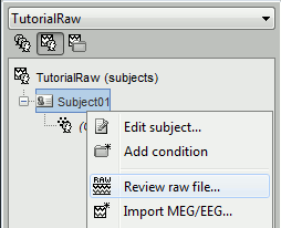
• Right-click on the subject node, and select: "Review raw file". Select the "Neuromag FIFF" file type, and open the only .fif file in the folder sample_mind_neuromag/data.
  
  

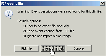
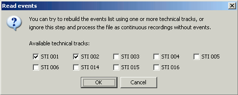
• A dialog window appears asking where to get the time markers (=events) from. Select "Event channel", and then "STI 001", to create a list of events based on the inputs that were recorded on the channel "STI 001".
  
  

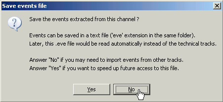
• Answer "No" to the question "Save the events extract from this channel?". Or you can say "yes" if you prefer, it doesn't really matter.
  
  

• A new folder with two files appears in the database explorer:
  
  

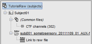
  • The channel file contains the definition of the sensors, exactly as when importing the files in the database with the "Import MEG/EEG" menu.
  • The node named "Link to raw file" contains all the information that was read from the continous file (file format, time vector, sampling frequency, events, bad channels, path to the original file, etc.), but no recordings. The MEG and EEG values recorded will be read directly from the native file, using the function in_fread.

Review the recordings

Open the file

Right-click on the data file > MEG (all) > Display time series.

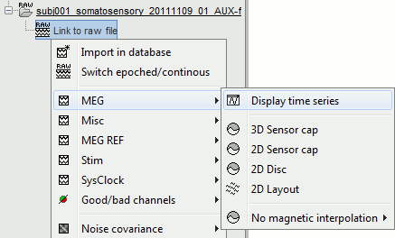
You can see a new tab "Event" and a time series figure.

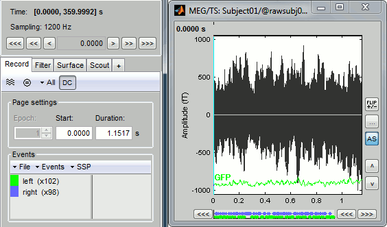
• Only a small block of the continuous recordings has been loaded in memory. This small time window can be modified with the tab "Event": the slider "Start" represents the beginning of the time window, and the text box "Samples" its length in number of time samples. The usual Brainstorm time controls (right-left corner of the main window) can be used to move the current time within that reduced time window.
• The panel "Recordings" in the Event tab lists the events that were detected on the "STI 001" input channel:
  • on the left, the groups of events (only one group here, Event #5, representing the electric stimulation of the right arm);
  • on the right, all the occurrences of the selected event group, described by the time instant at which they occur (here, the arm was stimulated 323 times).
• The time series figure is similar to the ones that were presented in the previous tutorials, with two new elements:
  • the events occurring in the current time window are shown at the top of the figure: if you click on a marker, it gets selected in the Event tab as well;

  • the navigation bar at the bottom represents the time of the entire raw file, where the events are also represented by smaller dots: The '<<' and '>>' buttons jump to the pervious/next segments, clicking on the bar change the current time window.

Channel setup

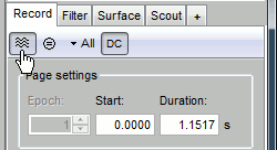
Let's switch to a nicer representation of the recordings time series: click on the "Display mode" button in the toolbar of the main Brainstorm window.

All the channels are displayed in the same figure, which makes it unreadable. Select a subset of channels by right-clicking on the figure > Display setup, or by using one of the keyboard shortcuts (Shift+A, B, C...).

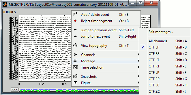
You can then adjust the vertical scale of the time series by holding the Shift key and moving the mouse wheel. The amplitude scale is represented on the right of the figure.

Adding/removing events

First create a group of events, define its name (test) and its color (red), with the "Events" menu in the Event tab:

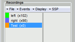
Then set the current time were you want to add a new Test even, by clicking on the figure (current time = where the vertical red line is). Select the group event "Test" and add a few occurrences with any of the three methods:

• In the Event tab: select the menu Events > Add event

• In the time series figure: right-click > Add event

• In the time series figure: press Control + A

Now remove all the events occurrences, but not the group "Test":

• In the Event tab: select one or more event occurrences (mouse click + Shift or Control), and press the "Delete" key.

• In the time series figure: click on the event to delete (on the blue dot), and right-click > Delete event

• In the time series figure: click on the event to delete, and press Control + A

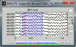
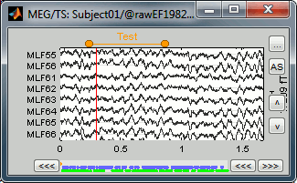
You can also use this interface to create events that have a temporal extension, ie. they last for more than one time sample. This is usually used to define bad/artifacted segments in the data.

• In the time series window, select a time range (click + move) instead of just setting the current time.
• Note that you can click outside of the white area to select the time (on top of the figure), in order not to select channels instead of moving.
• Add an event (menus or Control+A): note the way it is represented in the figure and in the Event panel.
• The first occurrence you add in an event group defines the event type: single time point, or time range. You cannot mix different types of events in a group.

Keyboard shortcuts

Select the event group "Event #5", then click on the time series figure and test all those shortcuts.

• Left / right arrows:

  • No other key: Change current time, sample by sample

  • With Control key: Change current time window (same as the "<<" and ">>" buttons)

  • With Shift key: Jump to next event of the selected group

• Page-up / page-down:

  • Same as left/right arrows, but faster.

  • If epochs are defined in the file: Control + page-up/page-down jumps to the next/previous epoch.

• Control + A: Add / delete event occurrence

• Control + T: Open a 2D topography window at the current time

• Shift + Letter: Changes the set of electrodes currently displayed in the figure (list available by right-clicking on the figure > Display setup > ...)

• Enter: Display the selected channels in a separate figure (selected channels = lines on which you clicked, that are shown in red)

• Escape: Un-select all the selected channels

• Delete: Mark the selected channels as bad

Mouse shortcuts

• Mouse click: Change current time

• Mouse click on a channel: Select the channel

• Mouse click + move: Select time range

• Mouse wheel: Zoom around current time

• Control + mouse wheel: Zoom vertically

• Shift + mouse wheel: Adjust the vertical scale of the time series

• Right-click: Display popup menu

• Right-click + move: Move in a zoomed figure

• Double click: Restore initial zoom settings (but do not restore the vertical scale of the time series)

Display options

When a block of recordings is loaded in memory, a few basic operations can be applied on it on the fly.

Event tab / Display menu

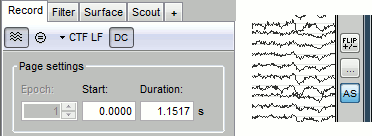
• Remove baseline: When selected, remove from each channel its average value over the entire current time window. This means that if you change the length of the time window, the value that is removed from each channel may change.

• Update amplitude scale: When selected, each time the time window changes, the vertical scale of the time series is adapted to the maximum value over the time window. When not selected: the vertical scales keeps its last value when you jump to another part of the file.

• Use CTF 3rd gradient compensation: Enable/disable the CTF noise-correction based on the reference sensors.

• Use Signal Space Projections: Apply/ignore the SSP vectors to the recordings, if some are available in the file.

Online filter

With the Filter tab in the main Brainstorm window, you can apply a band-pass filter to the recordings. Set the filter bounds and click on the Apply.

EEG Average reference

When reviewing EEG recordings, you can switch between the original values and the average reference by clicking on the "AVG REF" button in the toolbar of the main Brainstorm window.

Average reference computation: at each time point, the average of all the electrodes values is removed to each electrode.

Other views

Topography views

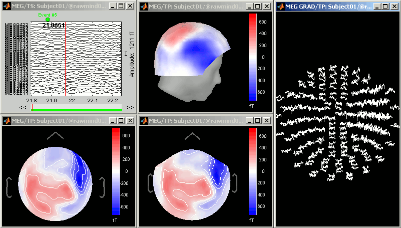
Exactly as introduced in the ?tutorial #4 "Exploring the recordings", you can display a variety of 2D/3D mappings of those recordings. Right-click on the node "Link to raw file" > MEG (all) > ...

Cortical sources

As presented in tutorial #5 to #7, you can compute successively for this raw file: a head model, a noise covariance matrix, and an inverse model.

• Head model: Keep the default anatomy and the default MRI / sensors registration, even though it is pretty bad: the goal of this tutorial is to illustrate what you can do with the raw file viewer in Brainstorm. Keep all the default options for the head model computation.

• Noise covariance matrix: Set as the baseline section the entire window before the first electric stimuation (the first occurrence of Event #5): for all those steps. Remember however that you can specify the time window to be considered as "noise" in the time window.

You will end with three new files as repre

Import in database

Save file

Import menus (x2)