Functions for Basic e-phys
Author: Konstantinos Nasiotis
The previous tutorials explained how to perform the spike sorting and the conversion to LFPs.
LFPs can be analyzed using the extensive library of methods from EEG and MEG research already present in Brainstorm. These signal processing libraries include artifact removal, time-frequency, connectivity, statistics and several other tools that are essential for analyzing electrophysiological data.
Spiking activity can be analyzed in a set of functions that is present in the Electrophysiology library, and help researchers understand their selectivity and interaction with the LFPs.
The figures in this page have been created with the spiking events that are initially available in the raw file. If you run one of the spike-sorters within Brainstorm you might get different events, leading to different visualizations.
Contents

Import LFP epochs
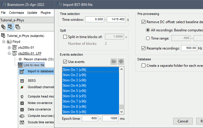
For the purpose of the tutorial, the timings around the presentation of the Superflow are selected as the segment of interest of the recordings. To import those segments: right-click on the LFP Link to raw file > Import in database.
- Select all the events of interest: 96 presentations * 9 event types ("Stim On" 1-9).
- Epoch time: -500ms - 1000ms
- Remove DC offset from all recordings
- Downsample to 500Hz: optional, but since LFP was filtered in the band 0.5-150Hz, the frequencies above 500Hz are not useful.
- Do not select the option "Create a separate folder"
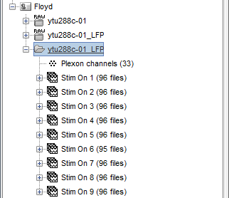
Note: As stated earlier on this tutorial, in order for the spiking functions to work, the spiking events should be named with the convention: “Spikes Channel ChannelLabel”. If the spike sorting is performed within Brainstorm, this should be done automatically. Users that import their own spiking events should organize their events in a compatible to Brainstorm format.
Tuning curves
The tuning curve is the most basic method of getting insights about neuronal selectivity in electrophysiology. Different conditions of a stimulus presentation are expected to elicit different number of spikes. Those conditions that each neuron is more “tuned” to, are expected to be recognized from a plot that shows that neuron’s number of spikes for each condition.
The tuning curves can be derived straight from the link to the raw file, since the events are already available in that file after the spike-sorting step. For computing the tuning curves, either the initial link to raw file or the link to the LFP file can be used.
- Drag and drop the Link to raw file to the process box
Run process Electrophysiology > Tuning Curves
Select the neurons and the conditions that should be displayed
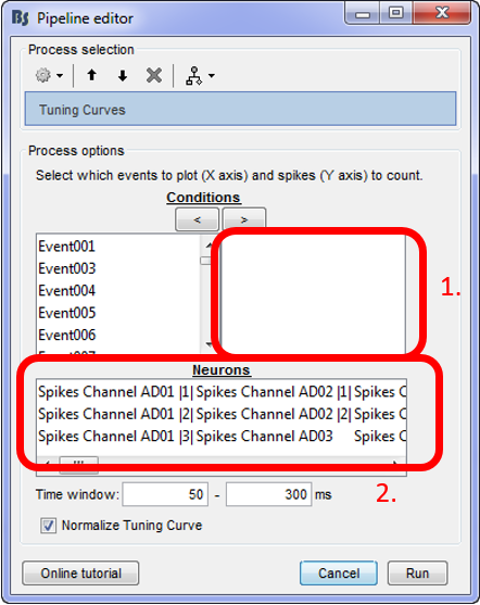
For using the tuning curve function, users have to make these selections:
Conditions: Since every experimenter uses their own event labels, the ordering of the stimulation events cannot be automated. Therefore, users have to select the order that they want to have their events on the x-axis (box 1). The events have to be selected and then the arrow that moves them in the right box according to the preferred ordering. Only the events in this box will be included in the Tuning Curves plot.
Neurons: The second step in this function, is for users to select the Neurons that the tuning curves will be computed for. A separate window will appear for each neuron.
Time window: The time-period around the events selected on step (i), that the spikes of each neuron selected will be counted.
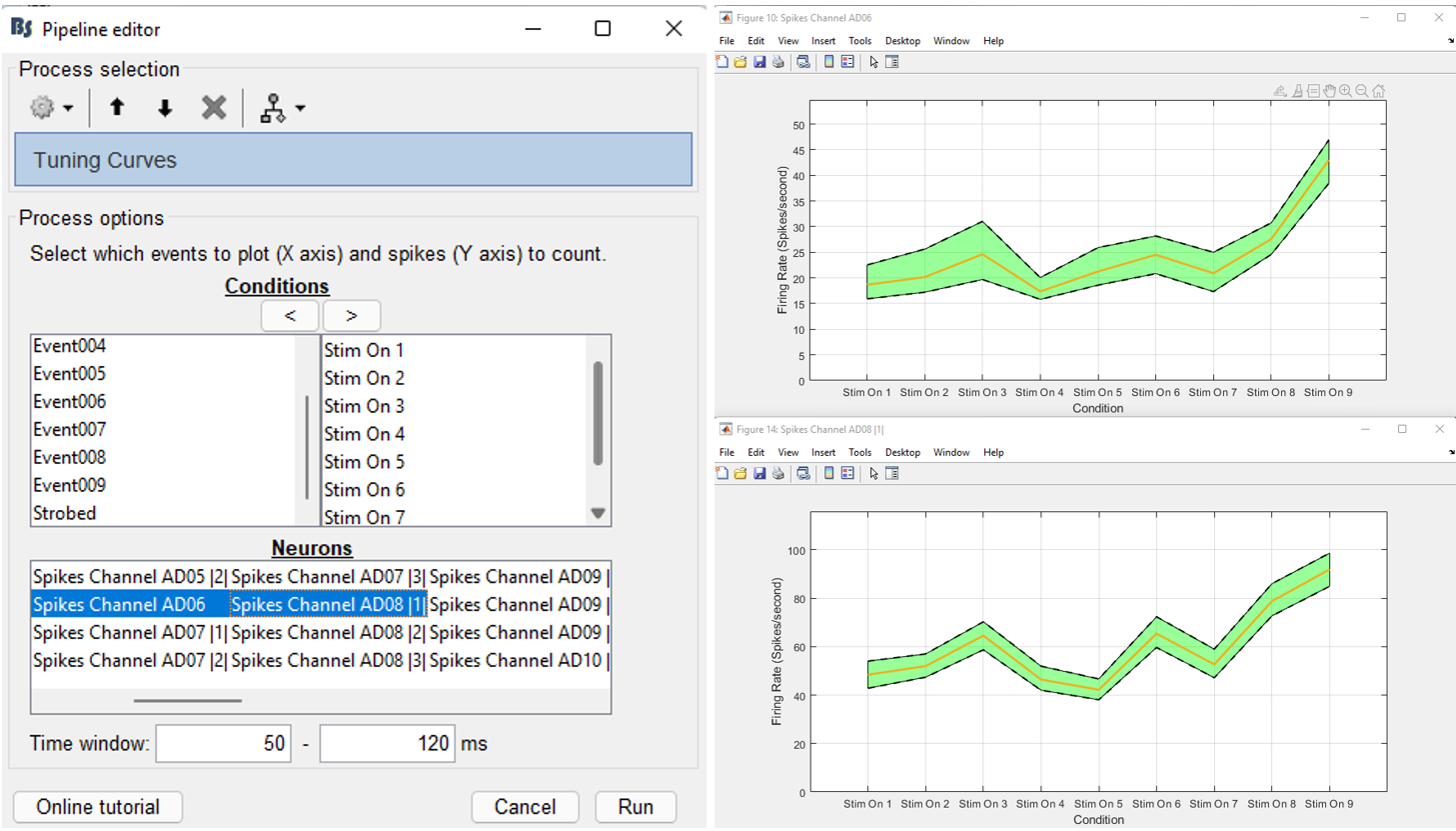
For the purpose of this tutorial, users should (considering the WaveClus spike sorting results):
- Select the Stim ON X events in a meaningful order
- Select the neuron from electrode AD06 and the first neuron from electrode AD08 (AD08 |1|)
- Select a time window between 50 and 120ms.
This will create two figures with the spatial selectivity of these two neurons on the selected conditions. The figures show the firing rate of the neurons on each condition, along with the 95% confidence intervals.
Noise correlation
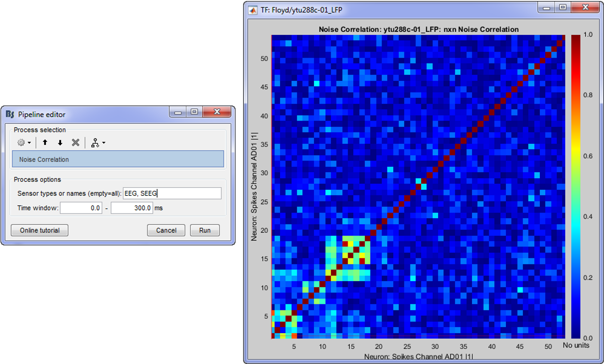
Correlation is a measure of the degree to which trial-to-trial fluctuations in response strength are shared by a pair of neurons. This is typically quantified as the Pearson correlation of the spike count responses to repeated presentations of identical stimuli under the same behavioral conditions (Cohen & Kohn 2011).
In Process1, select all the imported trials (see the first section of this page).
Run the process: Electrophysiology > Noise correlation.
- Adjust the Time window parameter
- The Pearson-correlation of all spike-trains from all neurons (some electrodes might pick up more than one neuron) will be computed after the baseline is removed and finally an NxN matrix (where N is the total number of neurons) will hold the noise correlation information.
References
Cohen MR, Kohn A, Measuring and interpreting neuronal correlations, Nature neuroscience, 2011
Spike field coherence
The spike-field coherence will effectively show the relationship between the spiking activity of a neuron, with the ongoing LFP oscillations as a matter of frequency. So, if a neuron is phase-locked to a specific frequency of the LFP oscillations, the SFC will show an increase only for that frequency. The computation of the SFC is based on the method from Fries et al. (2001). For more information users can check the supplementary figure 3 on the link listed at the end of this section.
In Process1, select imported trials for condition Stim On: 1.
Run process: Electrophysiology > Spike field coherence
Spike time window: The time-period around the spike-events. The LFP segments from all electrodes will be selected inside this window and the SFC will be computed in these segments
Parallel processing: Compute the FFT using a parfor loop. Greatly improves the speed of the process (requires Matlab's Parallel Processing toolbox).
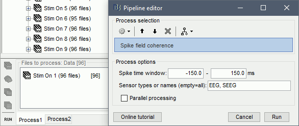
Once the computation is complete, double clicking on the created SFC icon will open the computed SFC for a single neuron. Each neuron can be selected from the drop-down box in the Display tab. The figure that appears, effectively shows the influence that the selected neuron has on all the electrodes on the recording, in all frequencies (up to the Nyquist limit).
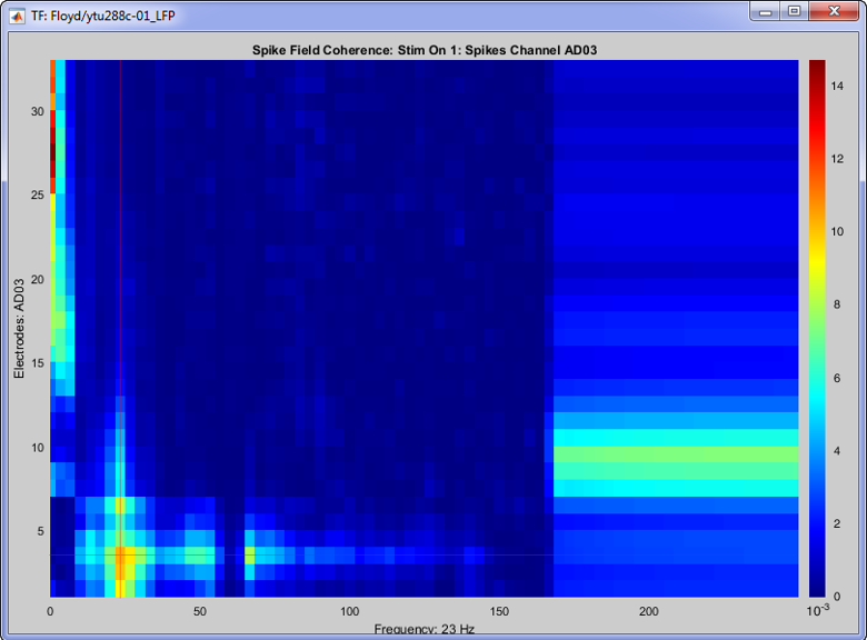
On the image above, the SFC from neuron 1 on channel with label “AD03” is shown for all 32 channels, for all frequencies up to 250 Hz (the trials were downsampled at 500 Hz, so we can get frequencies about to the Nyquist frequency). A clear cutoff frequency is shown above 150 Hz, since the LFP signals during the conversion were bandpass filtered at [0.5 - 150] Hz.
This neuron shows increased SFC on the Beta band and some high-gamma on the electrode that is picked up, and also some on the neighouring electrodes.
The increased low frequency SFC is ambigous due to the window selected around the spikes [-150,150] ms, and could be affected by edge-effects.
References
Fries P, Reynolds J, Rorie A, Desimone R, Modulation of oscillatory neuronal synchronization by selective visual attention, Science, 2001
Raster plot / Peristimulus time histogram
The raster plot/PSTH are basic methods for visualizing the selectivity of individual neurons. All trials are concatenated to display each neuron's behavior on all trials of a condition. These processes provide information on the selectivity but also the latency of the neurons on the experimental condition selected.
Raster plot per neuron
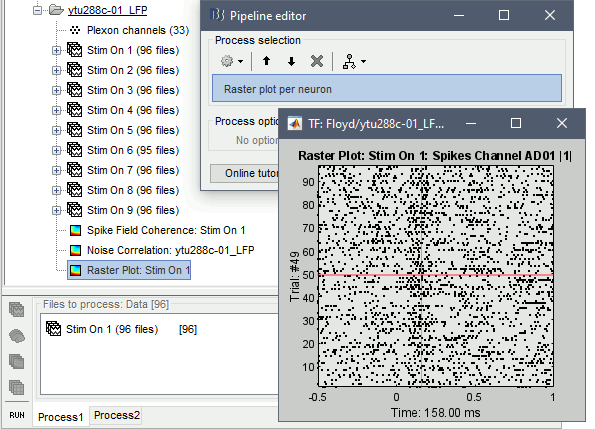
This function visualizes each neuron's spiking activity as a single dot for all trials selected. Users can select each individual neuron from the drop-down box in the Display tab. This function, does not use any binning (the x-axis is comprised with the same length as the time-samples of the trials).
In Process1, select imported trials for condition Stim On: 1.
Run process: Electrophysiology > Raster plot per neuron
The first neuron that was picked up on the electrode with label AD01 (Spikes Channel AD01 |1|) shows spiking latency ~120-180 ms after the stimulus presentation.
PSTH per neuron
This function computes the firing rate for all trials of a given condition, for each neuron. The bin size is a user-defined time-period and the spike-counts are computed and normalized for the bin-duration for each neuron.
This creates a matrix [Ntrials x Nbins] of the firing rates (where n is the number of trials and b the number of bins that fit the trial time-window). Users can select each individual neuron from the drop-down box in the Display tab.
In Process1, select imported trials for condition Stim On: 1.
Run process: Electrophysiology > PSTH per neuron
Spike time window: The bin size of the spiking histogram.
For the purpose of the tutorial, select a Bin size of 50ms.
The following figure shows the firing rate of some neurons increasing as a response to the stimulus presented (around 150-200 ms). Additionally, the bin at -75ms relative to the stimulus onset, there is a consistent increase on all neurons, indicative of the presence of an artifact within that bin.

For visualizing the 95% confidense intervals (1000 samples permutation test) of the firing rate of each bin, for each neuron, select the Butterfly visualization by right clicking on the display, and sequentially: Display options -> Display Mode -> Butterfly
PSTH per channel
(Binned firing rate per trial on the implanted topography)
We also included a second method that allows visualization of the binned spiking activity on the topography of the electrodes.
As with the previous PSTH plot method (PSTH per neuron), users have to define a bin-size where the spiking activity of each neuron will be computed. Since a single channel might record spiking activity from multiple neurons, this visualization will present only the firing activity for the first neuron. Therefore, for each condition, a separate file will be created for the first (or only) neuron that was picked up from that channel, containing the binned firing rates.
Users need to import the trials and sequentially Run > Electrophysiology > PSTH per Channel.
For the tutorial purposes, users should drag and drop the trials that correspond to condition Stim On: 1 to the process box and sequentially Run > Electrophysiology > PSTH per Channel.
This will create 96 binned trial files after the completion of the computations.
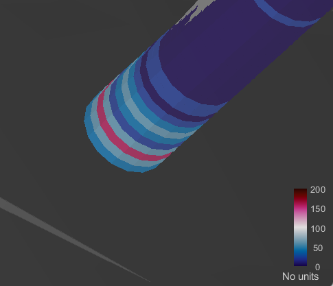
By right clicking on each of them and sequentially: SEEG -> 3D electrodes Head/Cortex/MRI 3D
users can visualize the firing rate activity on the implanted device and navigate through the binned trials. The smaller the bin size selected, the closer to real-time spiking activity one can get on the topography.
This visualization can be very helpful for monitoring propagating spiking activity across the implants.
Spike triggered average
The spike triggered average (STA) is a method for measuring the relation between the neuronal spiking and the local field potentials. If a neuron influences a distant electrode, the waveform of the STA should reveal these correlations. Effectively, this can be visualized with the averaging of the LFPs of all electrodes around the timing of a single neuron’s spiking and normalized by the spike-count.
In Process1, select imported trials for condition Stim On: 1.
Run process: Electrophysiology > Spike triggered average
Spike time window: The time-period around the spike-events. The LFP segments from all electrodes will be selected inside this window and the STA will be computed in these segments.
Parallel processing: Compute the FFT using a parfor loop. Greatly improves the speed of the process (requires Matlab's Parallel Processing toolbox).
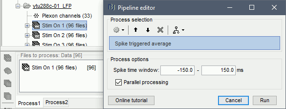
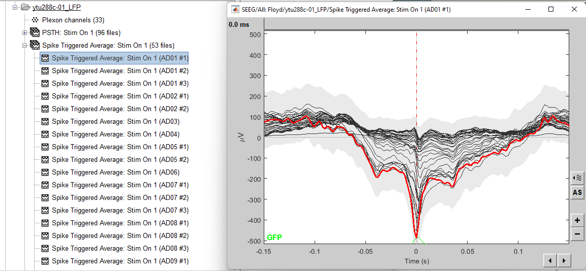
This process creates as many new files as individual neurons picked up from all electrodes (electrodes that picked up more than one neuron will create one file per neuron). The example below shows 70 new files created after the computation of the STA.
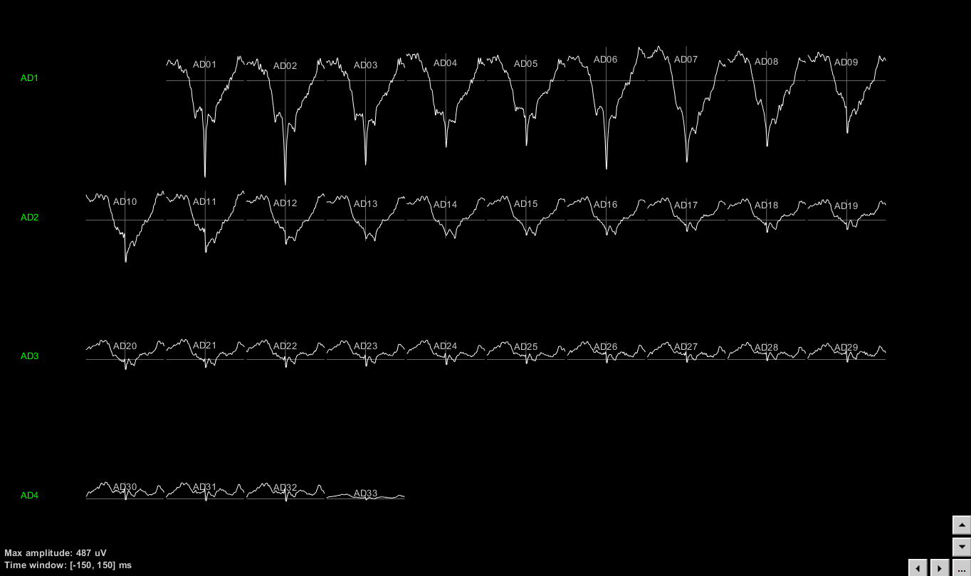
To display the STA on the implant geometry, users have to select one of the STA files, right click > SEEG > 2D Layout. Ctrl+E allows the display of the electrode labels. This menu is available only if the positions of the electrodes have been imported previously.
The following figure displays the STA for the neuron that was located on electrode AD01. It is clear that the LFPs close to the electrode that picked up the neuron are affected by this neuron’s firing. For easy navigation to the next neuron’s STA, press F3.
Spiking phase locking values
A hypothesis for how brain regions exchange information is through "communication by coherence" (Fries, 2005). The ongoing oscillations are hypothesized that create windows of opportunity for information exchange. Therefore, the relative timing of spiking activity to LFP oscillations of distant neuronal populations can encode stimulus information.
In Process1, select imported trials for condition Stim On: 9.
Run process: Electrophysiology > Spiking phase locking
Sensor types, indices, names or Groups: users can select the channel(s) of the ongoing oscillations. Users can select them based on their types (e.g. SEEG), indices (e.g. 1,10), names (e.g. AD01, AD02) or Groups: (group names that can be edited in the channel file)
Frequency band: Band-pass filtering of the selected signals
Phase binning: Size of each phase bin in degrees (total bins = 360/size_of_bins)
On this example, the oscillations in the alpha band for channel AD06 are selected for checking the spiking phase selectivity of all neurons from all channels.
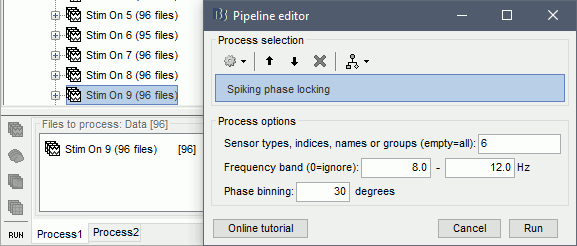
The function works in a multiplicative way: Phase locking values will be computed for all present neurons in the selected trials, for all selected sensors. e.g. for n Neurons and k channels, the dropdown will consist of n*k labels.
The following figure shows the phase selectivity of a neuron on channel AD06, relative to the ongoing alpha oscillations on the same channel.
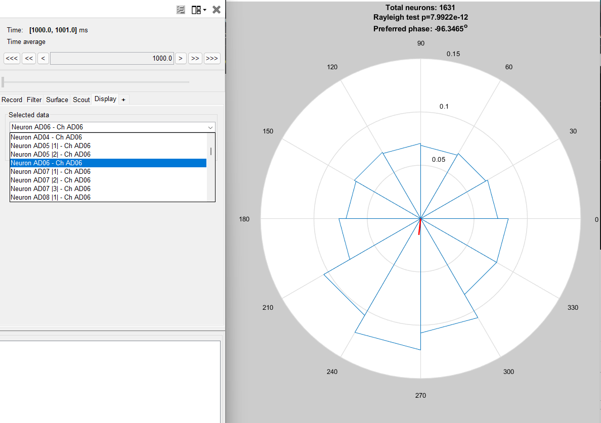
The total number of spikes for the selected neuron, the Rayleigh circular significance test, and the neuron's preferred phase are also displayed.
Reference
The function is using the circstat toolbox:
Berens P, CircStat: A MATLAB Toolbox for Circular Statistics, Journal of Statistical Software, 2009
Scripting
The following script from the Brainstorm distribution reproduces the analysis presented in this tutorial page: brainstorm3/toolbox/script/tutorial_ephys.m