Functions for Basic e-phys

Authors: Konstantinos Nasiotis

After performing the spike sorting and the conversion to the LFPs users have access to these invaluable types of information.

LFPs can be analyzed using the extensive library of methods that have been used in EEG and MEG research already present in Brainstorm. These signal processing libraries include preprocessing, artifact removal, time-frequency, connectivity, statistics and several other tools that are essential for analyzing electrophysiological data.

Spiking activity can be analyzed in a set of functions that is present in the Electrophysiology library (Run->Electrophysiology), and help researchers understand their selectivity and interaction with the LFPs.

For the purpose of the tutorial, the timings around the presentation of the Images are selected as the segment of interest of the recordings.

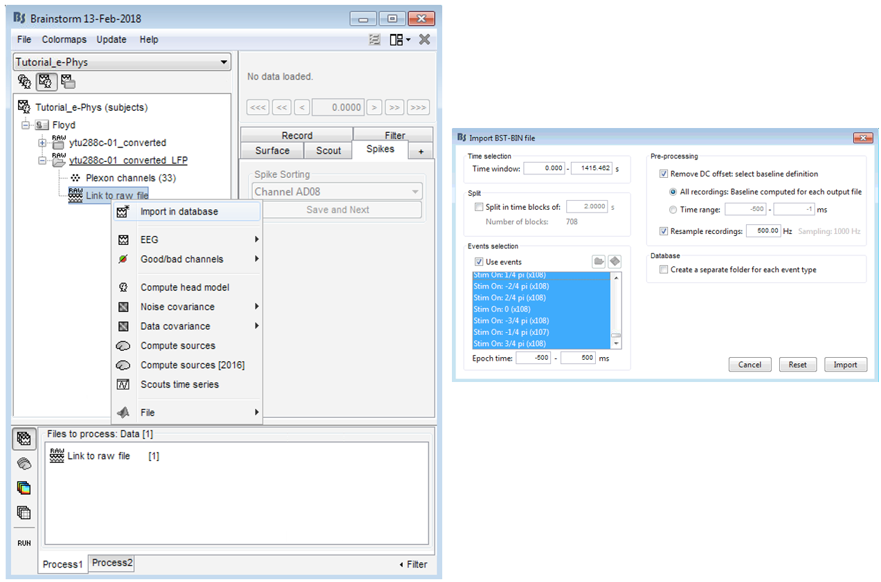
To import those segments, users should right click on the Link to raw file (On the LFP file)-> Import Recordings.

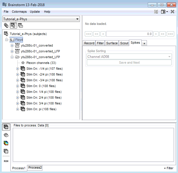
This will create 863 new entries in the database, since each event type (Stim On: …) was presented 108 times (Stim On -1/4 107 times).

All event types should be imported, as in the screenshot below:

Now that the trials are appropriately imported along with the spiking events in the database, users can use the functions that utilize them

Note: As stated earlier on this tutorial, in order for the spiking functions to work, they should be named with the convention: “Spikes Channel ChannelLabel”. If the spike sorting is performed within Brainstorm, this should be done automatically. Users that import their own spiking events should organize their events in a compatible to Brainstorm way.

Tuning Curves

The tuning curve is the most basic method of getting insights about neuronal selectivity in electrophysiology. Different conditions of a stimulus presentation are expected to elicit different number of spikes. Those conditions that each neuron is more “tuned” to, are expected to be recognized from a plot that shows that neuron’s number of spikes for each condition.

The tuning curves can be derived straight from the link to the raw file, since the events are already linked to that file after the spike-sorting step. For computing the tuning curves, either the initial link to raw file or the link to the LFP file can be used.

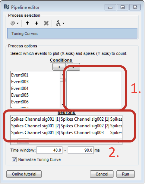
Users just need to drag and drop the Link to raw file to the process box, then click Run-> Electrophysiology->Tuning Curves. A new window will appear that allows users to select the neurons and the conditions that should be displayed.

For using the tuning curve function, users have to make these selections:

1. Conditions: Since every experimenter uses their own event labels, the ordering of the stimulation events cannot be automated. Therefore, users have to select the order that they want to have their events on the x-axis (box 1). The events have to be selected and then the arrow that moves them in the right box according to the preferred ordering. Only the events in this box will be included in the Tuning Curves plot.

2. Neurons: The second step in this function, is for users to select the Neurons that the tuning curves will be computed for. A separate window will appear for each window.

• The time-period around the events selected on step (i), that the spikes of each neuron selected will be counted.

4. Normalize tuning curve: If this checkbox is not selected, the tuning curves will just display the sum of the spike counts inside the selected time-window for each neuron. When selected, the tuning curves will be normalized based on the number of trials that each condition had.