Averaging the three unconstrained source directions for every scout

Dear Brainstorm users,

I want to average the three unconstrained source directions that I get for each scout and finally get only one source direction per scout.

My pipeline is:

  1. I place my unconstrained sources in the process 1 tab: Extract->Scout Time Series (I keep selected the mean function.)
  2. Then I place these time series in the process 1 tab: Average > Average signals > Average by scout (I keep selected either temporal PCA or mean function)

Temporal PCA seems to boost the time series with the maximum response, while mean function has the disadvantage of zeroing the signal when there are both positive and negative signals at the same time point (see example 2). I don't use mean(abs()) function, since the absolute value can alter tremendously the spectral contents of the signal and is not good for connectivity analysis.

Here are two examples:

Example 1:

Example 2:

What do you suggest I use: Temporal PCA or mean function?

Kind regards,
Konstantinos Tsilimparis

What do you suggest I use: Temporal PCA or mean function?

Our recent tests suggest that we should not use either approach.
The PCA damages the information contained in the signals. In simple simulations, the PCA approach was giving poorer results than using a constrained source model from the beginning.
Computing the mean of the three signals is equivalent to fixing an arbitrary direction (0,0,0)-(1,1,1) to all the dipoles - which does not make much more sense than using a constrained source model, which at least is based some physiological assumptions.

The only approach for the dimension reduction of these unconstrained source results that makes sense is using the norm of the vector at each location. However, this solution is not possible for connectivity analysis.

@Raymundo.Cassani is still working on our methodological recommendations for the for connectivity analysis of unconstrained source maps. We might end up recommending never flatting the source maps (to obtain one signal per location), and suggest two options:

  • computing the connectivity matrix for all the orientations (x,y,z), and take the maximum connectivity measure across the three orientations - which seems so far to give the best results.
  • using constrained sources instead.
1 Like

Thank you for your reply Francois!

So I decided to follow your advice about:

computing the connectivity matrix for all the orientations (x,y,z), and take the maximum connectivity measure across the three orientations.

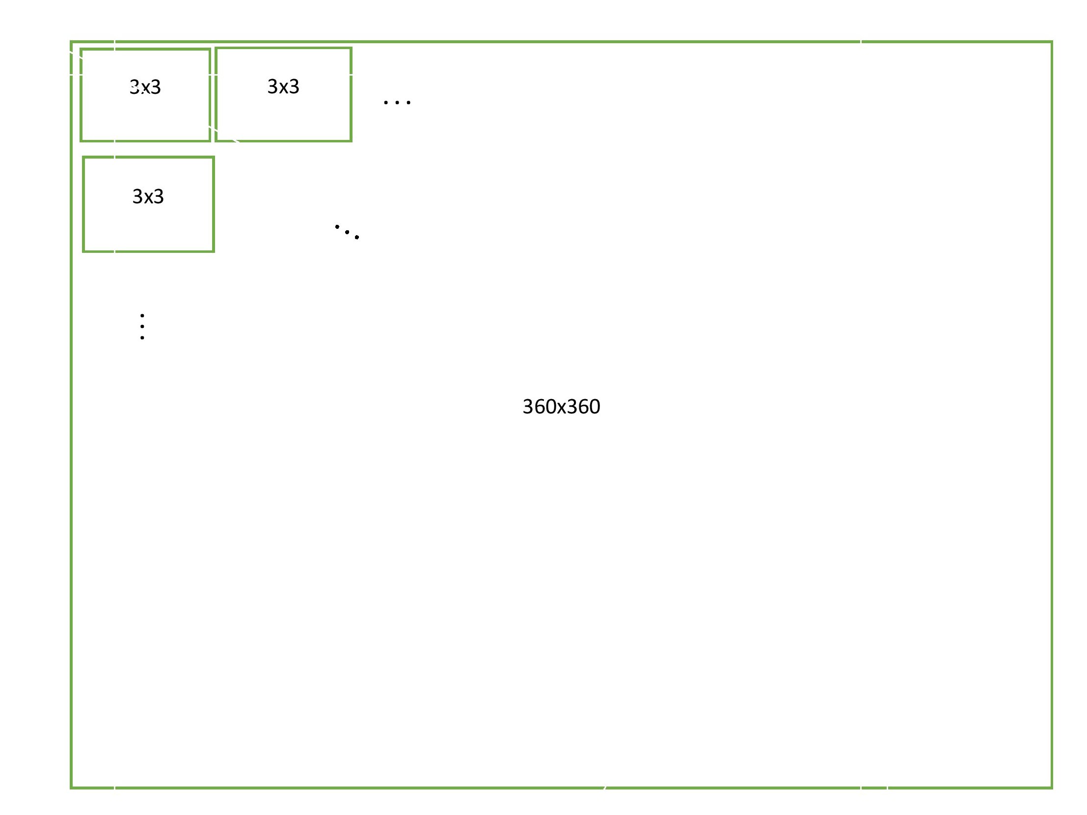
I work with AAL2 parcellation and I have 120 scouts. Because of the three source directions for each scout I get a 360x360 adjacency (connectivity) matrix.

In order to find the maximum connectivity measure for each xyz direction of each scout, I find the maximum value for all the 3x3 matrices inside the 360x360 adjacency matrix:

What do you think of this approach?

I will also upload my matlab script that does the aforementioned. It might be helpful for someone that needs to do a similar reduction in a adjacency matrix:

%% reducing the 3 source directions to 1 source direction per scout (matrix 360x360 becomes 120x120)
%% 3*43=129 adjacency matrices which means 43 subjects under 3 different conditions
%% Method used to find the adjacency matrices: Transfer Entropy (TE)

structure = load('TE.mat') ; %load structure
field=structure.indexes.TE.data; %load field

[rownum1,colnum1]=size(field);
[rownum,colnum]=size(field{1,1});

for i = 1 : rownum1
    for j = 1 : colnum1
        new_adjacency_matrix=zeros(rownum,colnum);
        adjacency_matrix=field{i,j}; % read the one of the 129 adj. matrices
        for k1 = 1:3:rownum-2 %1, 1+3=4 , ... , 155+3=158 -> 120 times
            for m1 = 1 : colnum
                Rows_Comparison = adjacency_matrix(k1:k1+2,m1);
                maximum=max(Rows_Comparison); %max(Rows_comparison) is a row vector 1x1 containing the maximum value of each column
                new_adjacency_matrix(k1,m1)=maximum; %create 360x360 matrix
            end
        end
        new_adjacency_matrix( ~any(new_adjacency_matrix,2), : ) = [];  %delete rows with zeros

%We have now a new_adjacency_matrix: 120x360

        for k2 = 1 : rownum/3 
            for m2 = 1:3:colnum-2 %1, 1+3=4 , ... , 355+3=358 -> 120 times
                Columns_Comparison = new_adjacency_matrix(k2,m2:m2+2);
                maximum=max(Columns_Comparison,[],2); %max(Columns_comparison) is a column vector 1x1 containing the maximum value of each row
                new_adjacency_matrix(k2,m2)=maximum; %create 120x360 matrix
            end
        end
        
        %Now we equate the columns: 2,3, 5,6, 8,9,... and so on with 0. That way we can get rid of them afterwards
        for k3 = 1 : rownum/3 
            for m3 = 1:3:colnum-2
                new_adjacency_matrix(:,m3+1)=0;
                new_adjacency_matrix(:,m3+2)=0;
            end
        end

        new_adjacency_matrix( :, ~any(new_adjacency_matrix,1) ) = [];  %delete columns with zeros
        TE_adjacency_matrix = new_adjacency_matrix- diag(diag(new_adjacency_matrix)); %make diagonal elements equal to 0
        save(['TE_adjacency_matrix_' num2str(i) '_' num2str(j) '.mat'],'TE_adjacency_matrix');

%We have now TE_adjacency_matrix: 120x120 with diagonal elements equal to 0

    end 
end

One question about this topic:

If I don't have the subject's anatomy I should use protocol´s default anatomy, and I read in the tutorial that when using default anatomy I should select the 'unconstrained' option for all the analysis, so, for now there is no way to compute an "accurate" source signal using the default anatomy? :open_mouth:

Will it work better if I select the "constrained" option despite I'm using a template brain?

Thanks in advances

What you describe is already what the connectivity processes do in Brainstorm, when you select "Apply scout function: Before" with unconstrained source maps in input. There is no need to develop anything more.

In @Raymundo.Cassani's experiments, we could observe that computing the average per ROI before computing the connectivity measure ("Scout function: before") degrades the quality of the estimation significantly. The best results seem to be obtained by computing the connectivity graph between all the individual vertices involved in all the ROIs, and then take the maximum across all the connectivity values between two ROIs. However, this becomes impractical for full-brain connectomes, as it requires computing matrices that can't fit in the memory of any regular computer (15000x15000xNfrequencies).

We are still actively discussing this topic, this is why our documentation takes so long to be published... We hope to get some clear recommendations in the next few weeks.

Indeed, this problem has been around for a decade, and we still don't have a clear solution for that.

For practicality, this is the solution I would personally favor. Even if a dipole of the source model is not in the best expected orientation, the cortex surface is so convoluted that there are always better dipoles in the near vicinity, and we can hope that most of the activity would be captured correctly somewhere (however, not exactly at the best possible location).
I guess that working with source models with orientations constrained to the cortex when this is not the correct brain shape increases the risk of positioning the peak activity a few vertices (~ a few mm, maybe up to 1cm) away from the actual peak, that we could localize with better modelling. However, it simplifies so much the post-processing for time-frequency or connectivity analysis, that this alternative is worth being considered.

If you need a very precise source localization, keep using an unconstrained model. The two options (constrained vs unconstrained) have different strengths.

1 Like

Thank you Francois!

I run the connectivity calculation for Phase Transfer Entropy NxN through brainstorm. I select the ''Apply scout function: before''. Hence I get a 120x120xfrequency bands adjacency matrix. However, this adjacency matrix doesn't have zero diagonal elements. Shouldn't this be fixed?

wow!
this reply really helps!
thanks a lot Francois! :slight_smile:

this adjacency matrix doesn't have zero diagonal elements

If you are using unconstrained sources, each diagonal is actually the maximum of 9 values: a 3x3 matrix with all the possible pairs with the 3 orientations. This is well explained in the new graphics @Raymundo.Cassani published in the cortico-muscular coherence tutorial:
https://neuroimage.usc.edu/brainstorm/Tutorials/CorticomuscularCoherence#Coherence_NxN_.28scout_level.29

Plus, are you sure the PTE of a signal with itself should be zero?
In general, the display in Brainstorm sets the diagonals of NxN connectivity matrices to zero to avoid the high values on the diagonal to drive the scaling of the colormap. By removing the highest values, we get a better representation capacity of the colormap.

It you still think their is something wrong with the diagonal values, please let me know and I'll investigate with the experts.

Dear Francois,

If the diagonal elements of the adjacency matrix are not equal to zero, then for example there could be information flow from the x-axis of scout-1 to the y-axis of scout-1. However, I personally believe that the diagonal elements of the adjacency matrix should be equal to zero, since there is no information flow from a scout to itself regardless of the scout's source direction.

I should note that when there are constrained sources, the diagonal elements of the adjacency matrix in Brainstorm are set equal to zero. Shouldn't that also be true for the unconstrained sources?

What do you believe?

Thank you,
Konstantinos

If the diagonal elements of the adjacency matrix are not equal to zero, then for example there could be information flow from the x-axis of scout-1 to the y-axis of scout-1.

Indeed. Since the signals are different along the X and Y directions, we compute a non-zero value.

However, I personally believe that the diagonal elements of the adjacency matrix should be equal to zero, since there is no information flow from a scout to itself regardless of the scout's source direction.

This is only a convention. If you don't want to see these non-zero diagonals, you can decide to ignore them. Alternatively, if they are really bothering you in the displays, you can explicitly set them to zero. This would require writing a script to edit the connectivity matrix saved in the TF field.
https://neuroimage.usc.edu/brainstorm/Tutorials/Connectivity#On_the_hard_drive

I should note that when there are constrained sources, the diagonal elements of the adjacency matrix in Brainstorm are set equal to zero. Shouldn't that also be true for the unconstrained sources?
What do you believe?

I don't believe in anything here. I just explained why you observe zero diagonals in the constrained case, and non-zero in the unconstrained case. At the moment, we don't have a better way to estimate the connectivity from unconstrained source maps. If this is not satisfying, as I already mentioned, you can use a constrained model instead: simpler data structures, simpler algorithms, possible minor loss in spatial accuracy (or fake impression of precision).

Hi Francois,

Just wanted to ask if there were any updates pertaining to the recommendations by the BST team?

Also, I am currently using constrained sources on a dataset that I do not have anatomical files for (so am using the ICBM152 template) to calculate AEC connectivity, but would like to compare these results to unconstrained sources. However, I am confused as to how to use the "max" function to get the max connectivity value per 3 orientations (e.g. reduce a 300 x 300 to 100 x 100 matrix when using 100 scouts). I compute the AEC on the unconstrained sources, but cannot select the "max" output, and the output is 100 x 100 matrix. I'm assuming this was done by taking the mean then of the 3 orientations per scout (I left it with the default options of mean and before)?

Thank you
Paul

Just wanted to ask if there were any updates pertaining to the recommendations by the BST team?

We have been working one these topics in the past months, but I'm not sure what your reference is.
I encourage you to review the tutorials below, which contains all the recommendations we have to share at the moment:

However, I am confused as to how to use the "max" function to get the max connectivity value per 3 orientations (e.g. reduce a 300 x 300 to 100 x 100 matrix when using 100 scouts).
I'm assuming this was done by taking the mean then of the 3 orientations per scout (I left it with the default options of mean and before)?

This is not an option, this is done automatically. The option you select is the scout function.
Please review carefully the explanations in this tutorial:
https://neuroimage.usc.edu/brainstorm/Tutorials/CorticomuscularCoherence#Method

Note that we do not give any recommendation on whether to use the option before vs. after. The is no consensus on this topic yet.
https://neuroimage.usc.edu/brainstorm/Tutorials/Connectivity

@Raymundo.Cassani Please correct me if I didn't report your recent conclusions correctly - Thanks.