Hello!
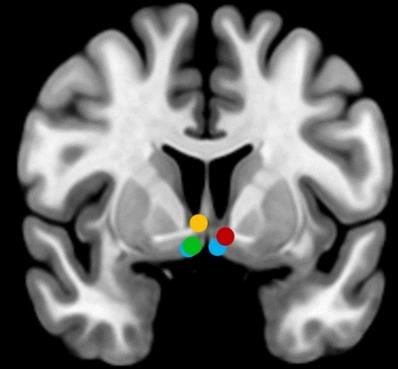
I collected the EEG data and used the source estimation in brainstorm. I mainly focus on the locations in picture 1.
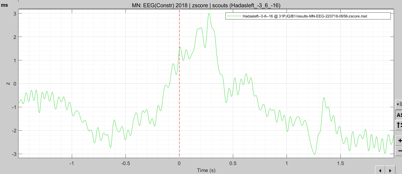
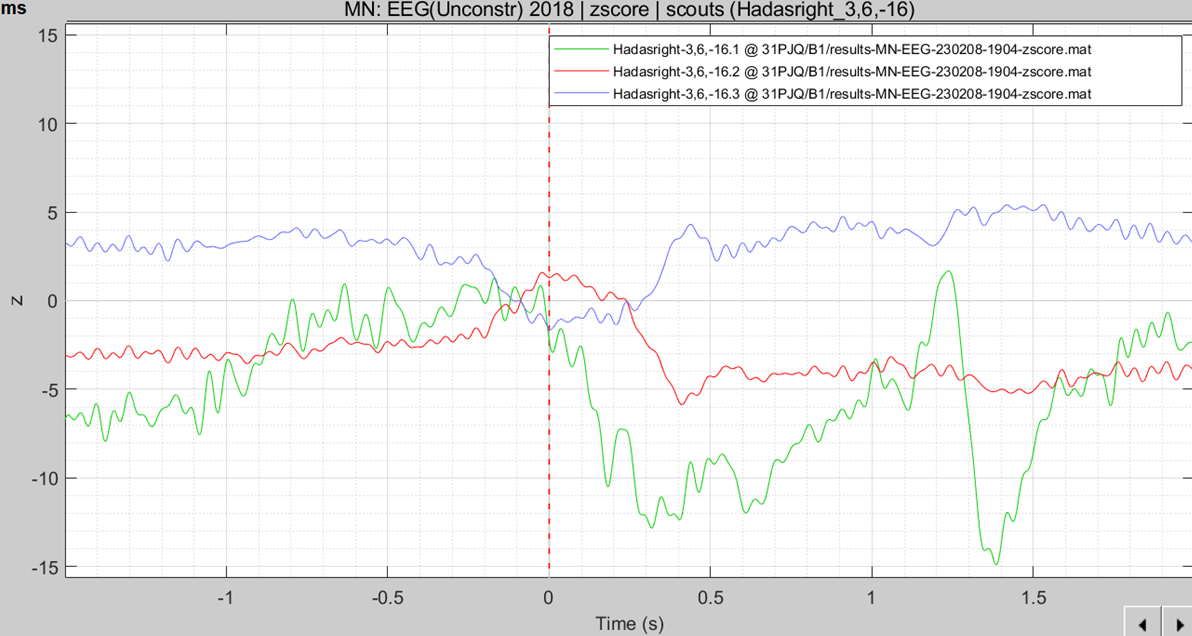
Here are the graphs of my source estimation results for the red point and blue point on the right side.
The result of red location is named as the 'd' picture.
The result of blue location on the right side is named as the 'b' picture.
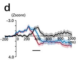
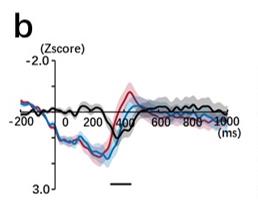
The red and blue lines in the 'b' and 'd' pictures, represent the GAIN and LOSS experiment condition separately. The black line is FRN, measured by LOSS minus GAIN. For the FRN, I am confused that why the source result is positive in the 'b' picture, but negative in the 'd' picture, even if the two loci are close to each other.
I would so appreciate if anyone can help.
The sign of the constrained source maps is discussed here:
https://neuroimage.usc.edu/brainstorm/Tutorials/SourceEstimation#Sign_of_constrained_maps
The sign of the difference between source maps is discussed here:
https://neuroimage.usc.edu/brainstorm/Tutorials/Difference
It is difficult to guide you with the interpretation of these results not knowing which methods you used.
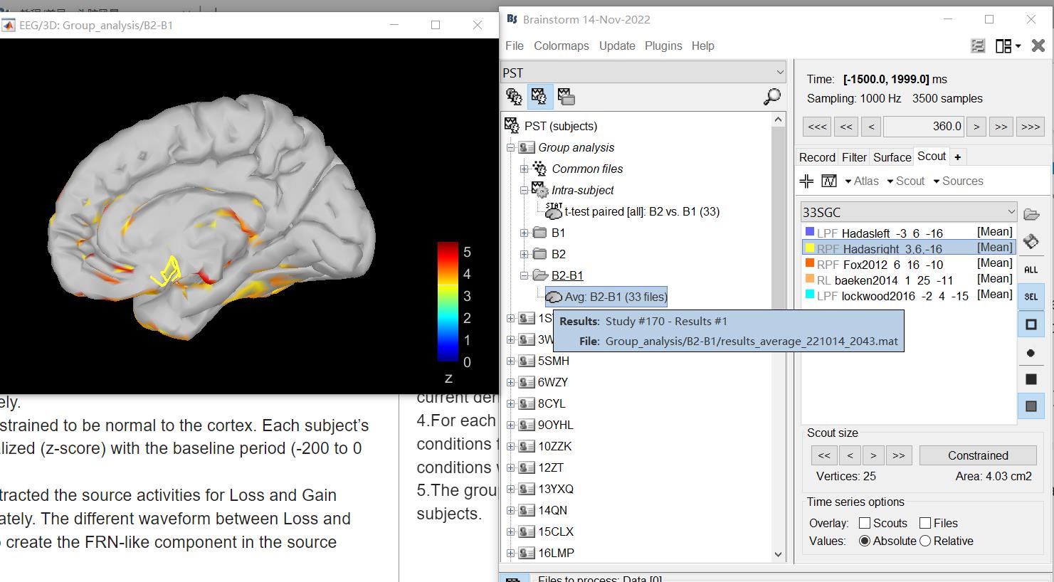
Also, if you want us to comment on your results, it would be better to provide screen captures of the Brainstorm graphics, including a screen capture showing the files in the database explorer.
Note that deep sources like these should be interpreted with caution. It is not obvious that EEG can capture signals from these deep brain regions, and if it does, the spatial precision you can expect from source modeling techniques is in the range of several centimeters. I'm not sure it is possible to distinguish between the various regions shown on your first image with EEG source estimation. The ERPs shown here are probably originated from more superficial sources.
Thanks for your reply!
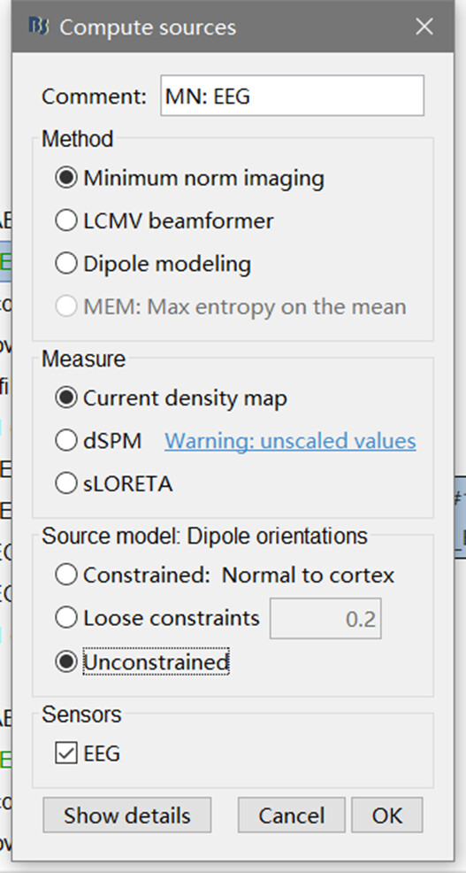
Here is the main procedure that I used:
1.The standard MNI template ICBM152 was used to create the head model, via the boundary element method implemented in OpenMEEG.
2.To obtain the source maps in loss and gain conditions, the current density maps were computed from the ERP time series using the minimum norm imaging for each condition in each subject separately.
3.The source orientation was constrained to be normal to the cortex. Each subject’s current density maps were normalized (z-score) with the baseline period (-200 to 0 ms).
4.For each region of interest, I extracted the source activities for Loss and Gain conditions for each subject separately. The different waveform between Loss and Gain conditions was calculated to create the FRN-like component in the source activities.
5.The group-wise Loss, Gain, and FRN-related source activity were averaged across all subjects.
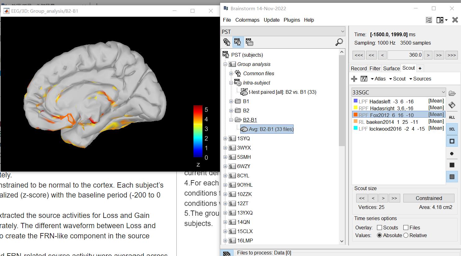
And here are the screenshots of the brain regions in brainstorm:
-
blue location on the right side ('b' picture):
-
red location ('d' picture):
With such deep sources, in EEG, you should expect adjacent sources to show very similar time series.
When using an anatomy template, the orientation of the sources cannot be trusted from the cortex surface. Additionally, in these central regions, the shape of the surface generated by FreeSurfer does not necessarily match the actual orientation of the cortex. Therefore the orientation constraints do not make much sense.
I recommend you use unconstrained sources instead, as recommended in the source estimation tutorials:
https://neuroimage.usc.edu/brainstorm/Tutorials/SourceEstimation#Unconstrained_orientations
Alternatively, you can use a volume head model. I recommend you try this on at least one pilot subject, this would give you a better feeling of the spatial precision you can expect from EEG source estimation:
https://neuroimage.usc.edu/brainstorm/Tutorials/TutVolSource
Hi, Francois!
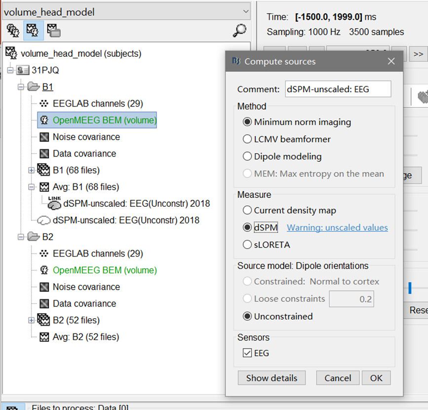
We tried the method you recommended, but we meet some problems.
When we used the orientation constraints and extra the scout time series, it generated one result. So it is easy to further analysis in MATLAB.
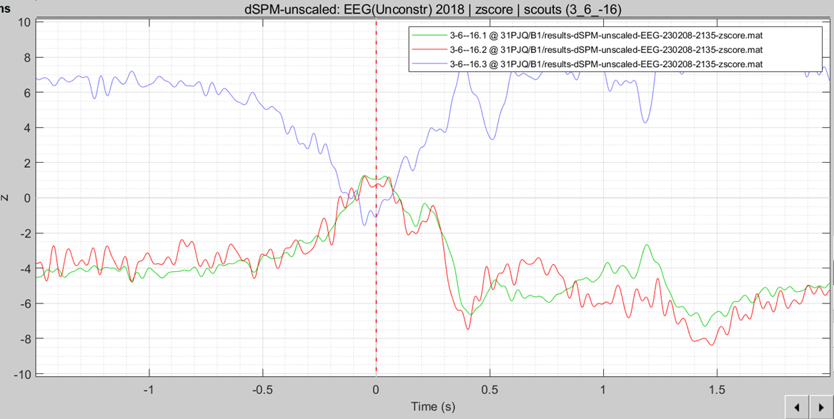
Then, we try to use the unconstrained sources and a volume head model, it generated three results. We read the tutorials, but still not understand which time series to select for further analysis and what is the criteria for selection.
With source models with no orientation constraints, the minimum norm solution includes three time series at each point of the grid, corresponding to dipoles in orthogonal orientations.
https://neuroimage.usc.edu/brainstorm/Tutorials/SourceEstimation#Unconstrained_orientations
This produces results that are possibly "less wrong" than models with orientations constrained to incorrect vectors, but that are more complicated to process as you have to deal with three signals instead of one.
If you need one signal and do not care about its phase, you can compute the norm of the three orientations ( sqrt(x^2 + y^2 + z^2) ).
Otherwise, you can try keeping only the first mode of the PCA along these three orientations. If you have questions relative to this topic: @Marc.Lalancette and @Sylvain are the experts.