Deviation maps

Authors: Pauline Amrouche, Lindsey Power, Raymundo Cassani

This tutorial introduces the implementation of the computation of deviation maps in Brainstorm. This tutorial is based on the results from five subjects of the OMEGA tutorial, as such, before proceeding, please complete the OMEGA tutorial as we will build on its results.

Introduction

Electrophysiology recordings have been used to estimate the brain activity, this is to say source estimation or source mapping. In this sense, several studies have explored the potential of electrophysiology-based source mapping to identify and describe abnormal activity patterns in patients with specific clinical phenotypes compared to healthy controls. Normative modelling has been used to define the healthy range of certain biomarkers and map individual differences at the single-subject level, a concept to which we refer as deviation maps. This approach has been applied in refractory epilepsy using scalp EEG in Janiukstyte et al., 2023 and in identifying new biomarkers for mild traumatic brain injury (mTBI) using MEG in Itälinna et al., 2023 for instance.

In this tutorial, we will create dummy deviation maps from the MEG spectral features of five subjects from the OMEGA tutorial. Four subjects will serve as the reference population, against which the fifth subject will be compared.

Pre-processing

Extract spectral features

Deviation maps can be derived from any statistic defined on a common spatial scale across subjects. For example, it is possible to extract spectral features from the power spectrum computed for each vertex of the cortical surface. These spectral features include the mean, standard deviation and coefficient of variation of the power spectra obtained across overlapping short-time windows. Note that the mean of these power spectra is by definition the power spectrum density (PSD) computed with the Welch method.

For this tutorial, we will compute the standard deviation of the power spectra from short-time windows with the process Compute PSD features. We will only use the first 100 s of the time series as it is faster and should lead to similar results. Then, we project those spectral results from each individual cortex to the common anatomy. The processing time for this step is around 6 minutes.

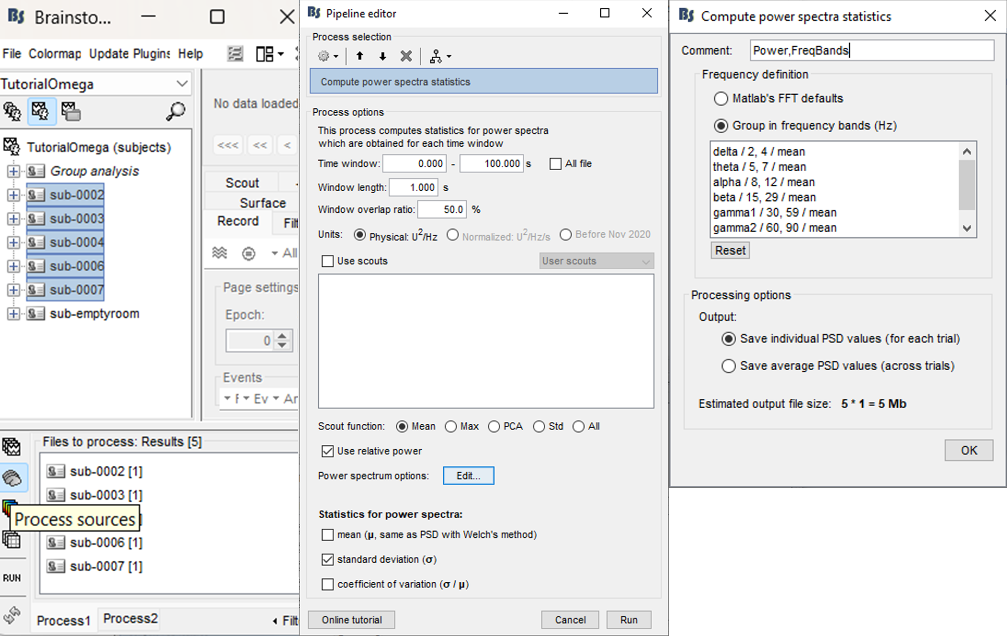
• Drag-and-drop the five subjects (not sub-emptyroom) into the Process1 box and click the [Process sources] button. You should have one file selected per subject.

• Select process: Frequency > Compute PSD features:

  • Time window: [0-100]s
    Segment of the time-series to be used.

  • Window length: 1s
    Short-time window length for which the power spectrum is computed.

  • Window overlap ratio: 50%
    Short-time window overlapping percentage.

  • Units: Physical U^2/Hz
    

  • Scouts: and Scout function: Uncheck
    To compute spectral features on Scouts.

  • Extract mean: Uncheck
    Whether to extract mean feature (across time windows), this is to say the PSD.

  • Extract std: Check
    Whether to extract standard deviation (across time windows).

  • Extract varcoef: Uncheck
    Whether to extract coefficient of variation (std/mean).

  • Use relative power: Check
    Whether the relative power (Power frequency bin / Total power) for each short-time window instead of the raw power of the frequency bin.

  • PSD options: Click
    Opens a panel to indicate the options of the FT.
    Frequency definition: Group in frequency bands
    Either the frequency definition is "continuous" or in bands. Click on reset to reset to the canonical frequency bands.
    Processing option: Save individual ...
    Either there is an output file per input file, or one output file as the average of all the individual output files.
    

The process Compute PSD features returns 1 to 3 files depending on the number of features extracted. This process shares several options with the process Frequency > Power spectrum density (Welch) process described in the PSD tutorial.

• 

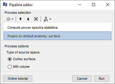
• Add process: Sources>Project on default anatomy: Cortex surface.
  

  • 

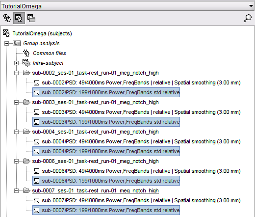
Once the processing is complete, you should see the one PSD file for the extracted PSD feature for each Subject folder in the Group analysis Subject.

• 

Deviation maps process

For each of the computed spectral files (standard deviation of power), there is a value for each vertex in the cortical surface and each frequency bin, thus the next step is to create a normative distribution from the values of the reference population (4 subjects in this example). For the one subject outside of this reference population, we calculate the z-score for the same feature relative to the normative distribution. When considering a given deviation level (d), the normative distribution is considered between the d/2​ and 1−d/2​ quantile interval of the reference distribution. For example, a deviation level of 0.05 leads to the quantiles at 2.5% and 97.5% of the reference distribution. If the feature value falls outside of those quantiles, we flag the (vertex-frequency) point as deviant. This process is repeated for every vertex and frequency, creating the frequency-defined deviation map.

We will now compute the deviation map for subject sub-0002 compared to the reference population (all other subjects).

• Click on the Process2 tab

• Drag-and-drop the file sub-0002/PSD: 199/1000ms Power,FreqBands std relative to the FilesA side of the Process2 tab. Which is located in the Subject Group analysis in the sub-0002_... folder.

• Similar to the step above, drag-and-drop the files sub-000X/PSD: 199/1000ms Power,FreqBands std relative for the remaining four subjects (sub-0003, sub-0004, sub-0006 and sub-0007) to the FilesB side of the Process2 tab.
  

  • 

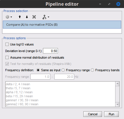
• Select process: Test > Compare (A) to normative PSDs (B) :

  • Use log10 values: Uncheck
    Whether log10 values of the feature are used.

  • Deviation level: 0.5
    Defines the normative distribution, see description in the above paragraph.

  • Assume normal distribution of residuals: Uncheck
    Whether consider the quantiles of a normal distribution rather than the quantiles of the empirical distribution.

  • Test for normality of residuals: Only available if assuming normal distributions
    If checked will output in the Brainstorm report the ratio of distributions for which the normality hypothesis can be rejected according to Shapiro-Wilk test. If the ratio is too high then the distributions should not be assumed normal.

  • Frequency definition: Same as input
    Definition of the frequency bands:
    Same as the input: use all frequency bins in input files.
    Frequency range: Subset of the original frequency axis in the input files.
    Frequency bands: Group frequency axis in bands, or subset of bands in the input files.
    

    

• Run the process.

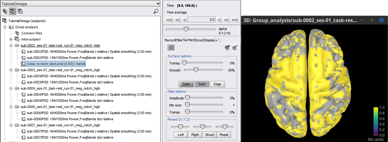
As result there will be a new PSD file: comp. to norm: devLevel (0.50) |  bands in the sub-0002_... folder.

• Open the file "comp. to norm: devLevel (0.50)| bands" for "comparison to normative, deviation level of 0.5, frequency bins by bands". This is the dummy deviation map for sub-0002, every vertex with value 1 falls outside of the desired quantiles of the normative distribution.
  

Additional documentation

• V. Janiukstyte et al., ‘Normative brain mapping using scalp EEG and potential clinical application’, Sci Rep, vol. 13, no. 1, p. 13442, Aug. 2023, https://doi.org/10.1038/s41598-023-39700-7.

• V. Itälinna, H. Kaltiainen, N. Forss, M. Liljeström, and L. Parkkonen, ‘Using normative modeling and machine learning for detecting mild traumatic brain injury from magnetoencephalography data’, PLOS Computational Biology, vol. 19, no. 11, p. e1011613, Nov. 2023, https://doi.org/10.1371/journal.pcbi.1011613.

Tutorials

• Tutorial: Source estimation

• Tutorial: Power spectrum

• Tutorial: Omega tutorial

• Tutorial: Statistics