Tutorial 10: Power spectrum and frequency filters
Authors: Hossein Shahabi, Francois Tadel, Elizabeth Bock, John C Mosher, Richard Leahy, Sylvain Baillet
We are now going to process our continuous recordings to remove the main sources of noise. Typically, we can expect contaminations coming from the environment (power lines, stimulation equipment, building vibrations) and from the subject (movements, blinks, heartbeats, breathing, teeth clenching, muscle tension, metal in the mouth or the body). In this tutorial, we will focus first on the noise patterns that occur continuously, at specific frequencies.
We can correct for these artifacts using frequency filters. Usually we prefer to run these notch and band-pass filters before any other type of correction, on the continuous files. They can be applied to the recordings without much supervision, but they may create important artifacts at the beginning and the end of the signals. Processing the entire continuous recordings at once instead of the imported epochs avoids adding these edge effects to all the trials.
Contents
- Evaluation of the noise level
- Interpretation of the PSD
- Elekta-Neuromag and EEG users
- Apply a notch filter
- Evaluation of the filter
- Some cleaning
- Note for beginners
- What filters to apply?
- When to apply these filters?
- Filter specifications: Low-pass, high-pass, band-pass
- Filter specifications: Notch
- Filter specifications: Band-stop
- On the hard drive
- Additional documentation
Evaluation of the noise level
Before running any type of cleaning procedure on MEG/EEG recordings, we always recommend to start with a quick evaluation of the noise level. An easy way to do this is to estimate the power spectrum of all the signals over the entire recordings.
- Clear the list of files in the Process1 tab.
Select the three datasets we have linked to our protocol.
You can select the three "link to raw file" nodes, the three folders or the entire subject node.

- Click on [Run] to open the pipeline editor window.
Select the process "Frequency > Power spectrum density (Welch)"
This process evaluates the power of the MEG/EEG signals at different frequencies, using the Welch's method (see Wikipedia or MathWorks). It splits the signals in overlapping windows of a given length, calculates the Fourier Transform (FFT) of each of these short segments, and averages the power of the FFT coefficients for all the overlapping windows.
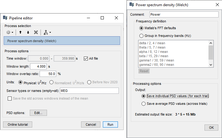
- Set the options as follows (click on [Edit] for the additional options):
Time window: [All file]
Portion of the input file you want to use for estimating the spectrum.
It is common to observe huge artifacts at the beginning or the end of the recordings, in this case you should exclude these segments from the calculation of the PSD.
In practice, using just the first 100s or 200s of the file can give you a good enough impression of the quality of the recordings.Window length: 4 seconds
Estimator length = length of the overlapping time windows for which we calculate the FFT. The number of time samples in the estimator is the same as the number of frequency bins in the output file. Increasing this parameter increases the output frequency resolution (distance between two frequency bins) but degrades the stability of the estimator, as it also decreases the total number of averaged time windows. A Hamming window is applied to each estimator window before the computation of the FFT. See forum post: Effect of window length on the PSDOverlap: 50%
How much overlap do we want between two consecutive time windows.Units: Physical: U^2/Hz
Scaling of the spectrum. This only affects the values on the Y axis of the spectrum. Physical units should be used in most cases.
"Normalized" gives normalized frequencies from 0 to 2pi (Hz·s).
"Before Nov 2020" reproduces the older Brainstorm spectrum scaling (see this forum post).Sensor types or names: MEG
Defines the list of channels (names or types) on which you want to apply the process.Frequency definition: Matlab's FFT default
You have the option to directly use the frequency binning returned by the FFT, or run an additional step of averaging these bins in larger frequency bands. Note that you can freely edit these frequency bands.Output: Save individual PSD value.
This option will separately estimate the PSD for each of the three files in input, and create three files in output. If you select the other option (save average), it calculates the same three files but averages them on the fly and saves only one file in the database.Implementation details: See function brainstorm3/toolbox/timefreq/bst_psd.m
- Click on [Run] to start the execution of the process.
Troubleshooting: If you get "Out of memory" errors, try to run this PSD estimation on a shorter time segment. For example, set the time window to [0,100s] instead of the full file. This process starts by loading all the needed recordings in memory, you might not have enough memory available on your system to fit the entire dataset.
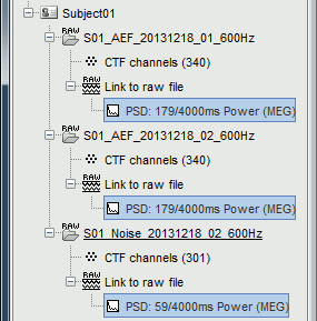
It produces three new files, that appear as "depending" on the three datasets. The comments of the files indicate how many overlapping windows could be used to estimate the PSD. "179/4000ms" means 179 windows of 4s each (total 716s). With the 50% overlap, it sums up to a little less than 2x the file length (360s).
Interpretation of the PSD
File: AEF#01
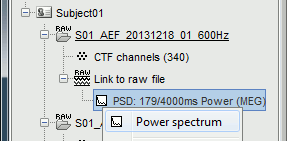
Double-click on the new PSD file for run #01 to display it (or right-click > Power spectrum).
- The power spectrum is displayed in a figure similar to the time series, but the X axis represents the frequencies. Most of the shortcuts described for the recordings are also valid here. Clicking on the white parts of the figure or using the arrow keys of the keyboard move the frequency cursor. The current frequency can also be controlled with a new slider displayed in the Brainstorm window, just below the time panel.
Each black line represents the power spectrum for one channel. If you click on a channel, it gets highlighted in red. Click again for deselecting. Right-click on a selected channel to read its name.
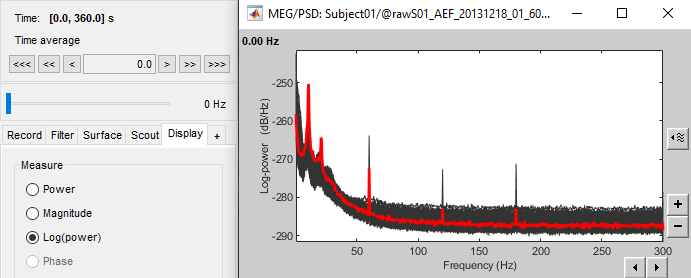
The frequency resolution of this power spectrum, ie. the distance between two frequency bins represented in this figure, is about 0.15Hz. This precision depends on the length of the estimator window you used. The FFT is computed on the number of time samples per window (4s*600Hz), rounded to the next power of 2 (nextpow2), and represents the full spectrum of the file (0-600Hz).
Frequency resolution = sampling_freq / 2^nextpow2(estimator_length*sampling_freq) = 0.1465 Hz- The shape of this graph is normal, it does not indicate anything unexpected:
Peaks related with the subject's alpha rhythms: around 10Hz and 20Hz.
Peaks related with the power lines: 60Hz, 120Hz and 180Hz.
These datasets were recorded in Canada, where the alternating powerline current is delivered at 60Hz. In Europe you would observe similar peaks at 50Hz, 100Hz and 150Hz.
- Add a topography view for the same file, with one of the two methods below:
Right-click on the PSD file > 2D Sensor cap.
Right-click on the spectrum figure > 2D Sensor cap (shortcut: Ctrl+T)
Scroll in frequencies to see the spatial distribution of each frequency bin:

- We have already identified two artifacts we will need to remove: the eye movements and the 60Hz+harmonics from the power lines.
File: AEF#02
Open the spectrum view for the run AEF#02.
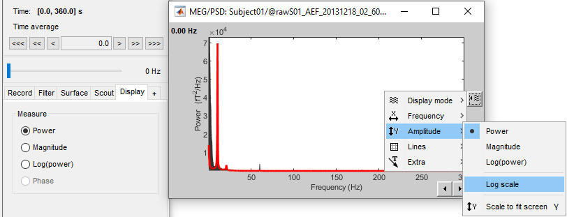
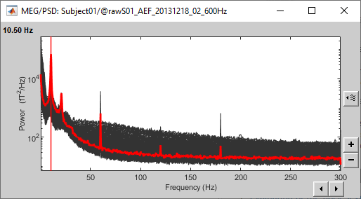
To view the signal units instead of dB, select Display Tab > Measure > Power. Then from the display options icon on the right of the figure, select Amplitude > Log scale
Add a 2D sensor cap view for the same file. Scroll to zoom in/out.
To display the sensor names, right-click on the figure > Channels > Display sensors.- This spectrum looks very similar to the run #01: same alpha and power line peaks.
Additionally, we observe higher signal power between 30Hz and 100Hz on many occipital sensors. This is probably related to some tension in the neck muscles due to an uncomfortable seating position in the MEG. We will see later whether these channels need to be tagged as bad or not.

File: Noise recordings
Open the spectrum view for the noise recordings.
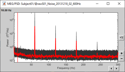
- This shows the power spectrum of the signals that are recorded when there is no subject in the MEG room. It gives a good and simple representation of the instrumental noise. If you had one bad MEG sensor, you would see it immediately in this graph. Here everything looks good.
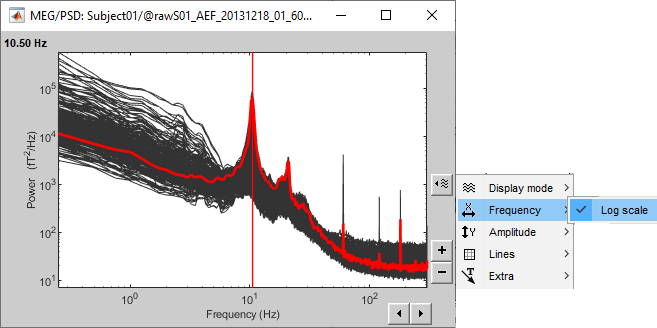
X Log-scale
One option is worth mentioning when displaying power spectra: the logarithmic scale for the X axis. In the diaply options for the PSD figure > Frequency > Log scale. It is sometimes better adapted to represent this type of data than a linear scale (especially with higher sampling frequencies).
Elekta-Neuromag and EEG users
The Elekta-Neuromag MEG systems combine different types of sensors with very different amplitude ranges, therefore you would not observe the same types of figures. Same thing for EEG users, this might not look like what you observe on your recordings.
For now, keep on following these tutorials with the example dataset to learn how to use all the Brainstorm basic features. Once you're done, read additional tutorials in the section "Other analysis scenarios" to learn about the specificities related with your own acquisition system.
Apply a notch filter
This filter has been updated in 2019. In the new configuration, the user can define the 3-dB bandwidth of the filter. Please consider that a smaller bandwidth means a sharper filter which in some cases makes filter unstable. In case you want to reproduce the old filter, you can check the box "Use old filter implementation". The 3-dB bandwidth is not applicable to the old configuration.
For illustration purposes, we will now run a frequency filter to remove the 60Hz+harmonics from the continuous files. Notch filters are adapted for removing well identified contaminations from systems oscillating at very stable frequencies.
Keep all the three datasets selected in the Process1 box.
Remember to always apply the same filters on the subject recordings and the noise recordings.- Click on [Run] to open the Pipeline editor.
Run the process: Pre-process > Notch filter
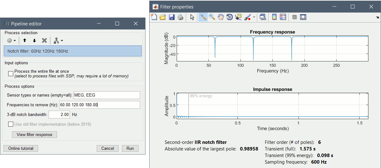
Process the entire file at once: NO
Sensor types or names: MEG
Frequencies to remove: 60, 120, 180 Hz
3-dB notch bandwidth: 2 Hz
- The higher harmonics (240Hz) are not clearly visible, and too high to bother us in this analysis.
This process creates three new datasets, with additional "notch" tags. These output files are saved directly in the Brainstorm database, in a binary format specific to Brainstorm (.bst).
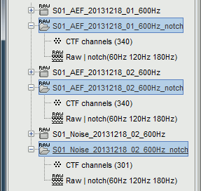
- If you delete the folders corresponding to the original files (before the filter), your original recordings in the .ds folders are not altered. If you delete the folders corresponding to the filtered files, you will lose your filtered recordings in .bst format.
To check where the file corresponding to a "Link to raw file" is actually saved on the hard drive, right-click on it > File > Show in file explorer.
Important: This is an optional processing step. Whether you need this on your own recordings depends on the analysis you are planning to run on the recordings (see advanced sections below).
Evaluation of the filter
Right-click on the Process1 list > Clear list.
Drag and drop the three filtered files in Process1.
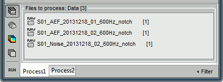
Run again the PSD process "Frequency > Power spectrum density (Welch)" on the new files, with the same parameters as before, to evaluate the quality of the correction.
Double-click on the new PSD files to open them.
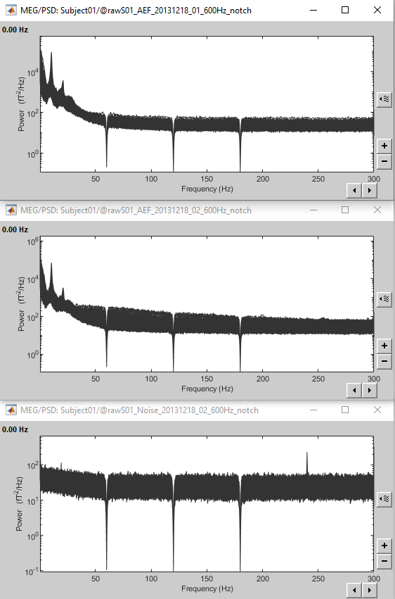
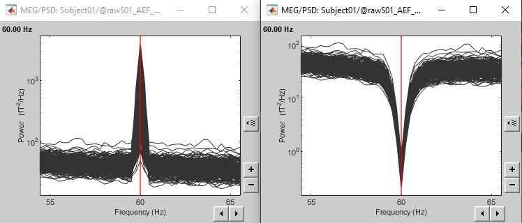
Scroll to zoom in and observe what is happening around 60Hz (before / after).
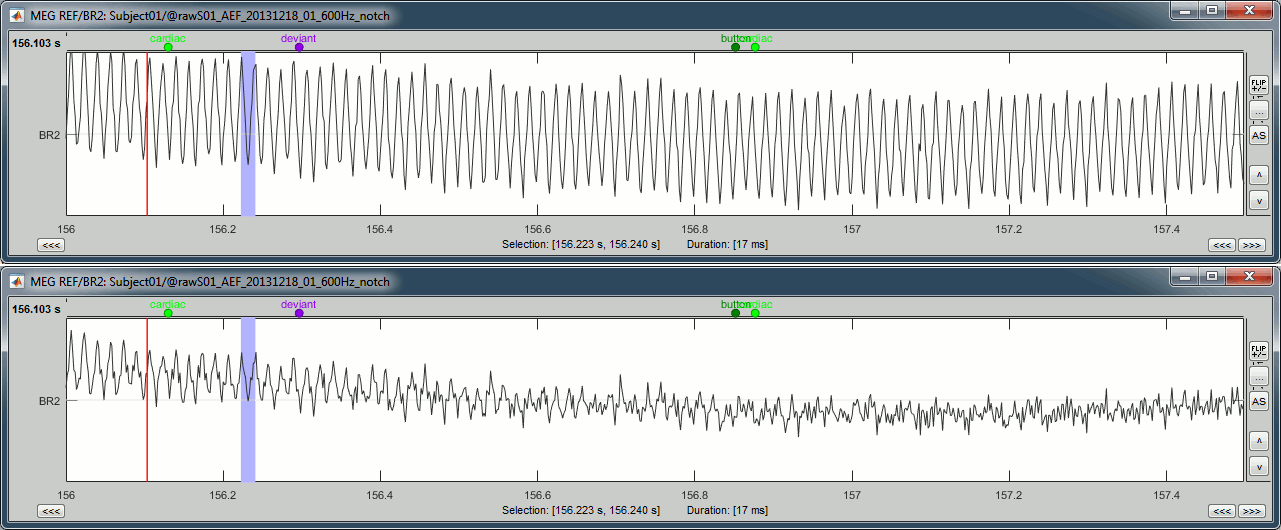
See below an example of how this filter can affect the time series: top=before, bottom=after.
We show the reference sensor BR2 because it shows a lot more 60Hz than any MEG sensor (sensor type "MEG REF"), ie. oscillations with a period of 16.7ms.
Note the edge effect at the beginning of the signal: the signals below are 1.5s long, the notch filter at 60Hz is visibly not performing well during the first 500ms (blue window).
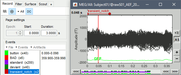
If you look in the list of events, you would see a new category "transient_notch". This corresponds to the time period during which can expect significant edge effects due to the filtering. Brainstorm doesn't mark these blocks as bad by default, you would have to do it manually - you will see how to do this in one of the following tutorials. In the case of this dataset, the transient duration is much shorter than the delay before the first stimulation, so not relevant in our processing pipeline. See the advanced sections below for more details about the estimation of this transient duration.
Some cleaning
To avoid any confusion later, delete the links to the original files:
Select the folders containing the original files and press Delete (or right-click > File > Delete).
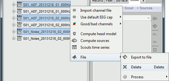
Always read the confirmation messages carefully, you will avoid some bad surprises.

This is what your database explorer should look like at the end of this tutorial:
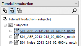
Note for beginners
Everything below is advanced documentation, you can skip it for now.
What filters to apply?
The frequency filters you should apply depend on the noise present in your recordings, but also on the type of analysis you are planning to use them for. This sections provides some general recommendations.
High-pass filter
Purpose: Remove the low frequencies from the signals. Typically used for:
Removing the arbitrary DC offset and slow drifts of MEG sensors (< 0.2Hz),
Removing the artifacts occurring at low frequencies (< 1Hz, e.g. breathing or eye movements).
Warnings:
- Edge effects: Transient effects you should discard at the start and end of each filtered signal because the filtering window extends into time periods outside those for which you have data.
- Avoid using on epoched data: You need long segments of recordings to run a high-pass filter.
- Be careful with the frequency you choose if you are studying cognitive processes that may include sustained activity in some brain regions (eg. n-back memory task).
Low-pass filter
Purpose: Remove the high frequencies from the signals. Typically used for:
- If the components of interest are below for example 40Hz, you may discard the faster components in the signal by applying a low-pass filter with a frequency cutoff below 40Hz.
- Removing strong noise occurring at high frequencies (eg. muscle contractions, stimulators).
- Display averages: In an event-related design, you will import and average multiple trials. You may low-pass filter these averages for display and interpretation purposes.
- Statistics: In an event-related study with multiple subjects, the latency of the brain response of interest may vary between subjects. Smoothing the subject-level averages before computing a statistic across subjects may help reveal the effect of interest.
Warnings:
- Edge effects: Transient effects you should discard at the start and end of each filtered signal because the filtering window extends into time periods outside those for which you have data.
- It is always better to filter continuous (non-epoched data) when possible.
- When filtering averages: Import longer epochs, average them, filter, then remove the beginning and the end of the average to keep only the signals that could be filtered properly
Band-pass filter
Purpose: A band-pass filter is the combination of a low-pass filter and a high-pass filter, it removes all the frequencies outside of the frequency band of interest.
Warnings: The same considerations and warnings as for high and low pass filtering apply here.
Notch filter
Purpose: Remove a sinusoidal signal at a specific frequency (power lines noise, head tracking coils).
Warnings:
- Use only if needed: It is not always recommended to remove the 50-60Hz power lines peaks. If you don't have a clear reason to think that these frequencies will cause a problem in your analysis, you don't need to filter them out.
- In an ERP analysis, the averaging of multiple trials will get rid of the 50-60Hz power line oscillations because they are not time-locked to the stimulus.
- If you are using a low-pass filter, do not a apply a notch filter at a higher frequency (useless).
Alternatives: If the notch filter is not giving satisfying result, you have two other options.
Band-stop filter: Similar to the notch filter, but more aggressive on the data.
Useful for removing larger segments of the spectrum, in case the power line peaks are spread over numerous frequency bins or for suppressing other types of artifacts.Sinusoid removal: This process can do a better job at removing precise frequencies by identifying the sinusoidal components and then subtracting them from the signals in the time domain. This is not a frequency filter and works best on short segments of recordings.
Run it on the imported epochs rather than on the continuous files.
When to apply these filters?
Continuous files: Frequency filters used for pre-processing purposes should be applied before epoching the recordings. In general, filters will introduce transient effects at the beginning and the end of each time series, which make these parts of the data unreliable and they should be discarded. If possible, it is safer and more efficient to filter the entire recordings from the original continuous file at once.
Before SSP/ICA cleaning: Artifact cleaning with SSP/ICA projectors require all the channels of data to be loaded in memory at the same time. Applying a frequency filter on a file that contains projectors requires all the file to be loaded and processed at once, which may cause memory issues. Pre-processing filters are rarely changed, whereas you may want to redo the SSP/ICA cleaning multiple times. Therefore it is more convenient to apply the filters first.
Imported epochs: Filtering epochs after importing them in the database is possible but requires extra attention: you may need to import longer epochs to be able to deal with the edge effects.
After averaging: You may low-pass filter the averaged epochs for display or statistical purposes but again be aware of the edge effects.
Empty room measurements: In principle, all the filters that are applied to the experimental data also need to be applied, with the same settings, to the noise recordings. In the source estimation process, we will need all the files to have similar levels of noise, especially for the calculation of the noise covariance matrix. This applies in particular when some channels are noisy.
Think first: Never apply a frequency filter without a clear reason (artifacts, predefined frequency ranges of interest, etc.) and without keeping the side effects under control. Avoid when possible.
Filter specifications: Low-pass, high-pass, band-pass
Process: Pre-process > Band-pass filter
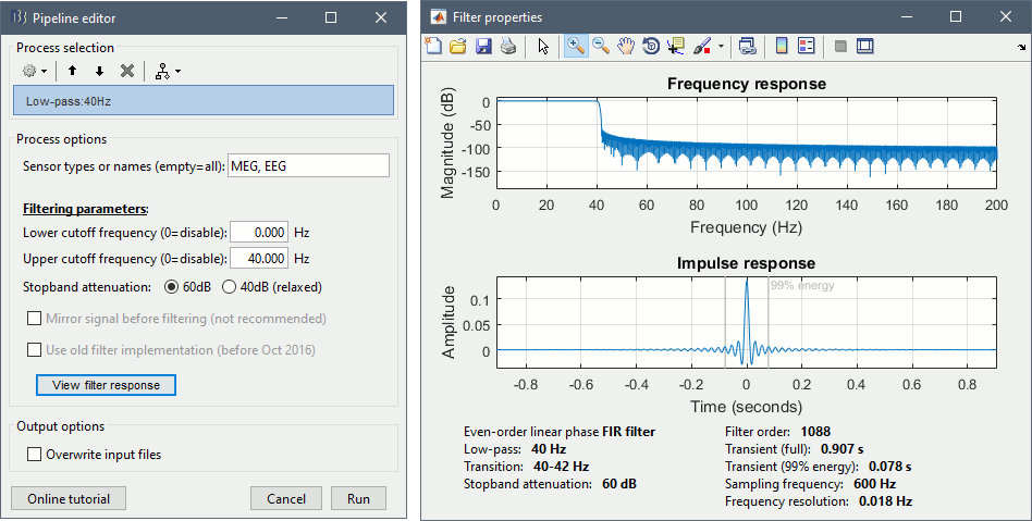
Process options:
Lower cutoff frequency: Defines a high-pass filter (enter 0 for a low-pass filter)
Upper cutoff frequency: Defines a low-pass filter (enter 0 for a high-pass filter)
Stopband attenuation: The higher the attenuation, the higher the performance of the filter, but longer the transient duration. Use the default (60dB) unless you need shorter edge effects.
Use old filter: For replicating results obtained with older versions of Brainstorm.
View filter response: Click on this button to display the impulse and frequency response of your filter, and confirm that the responses appear reasonable.
Filter design:
Description: Even-order linear phase FIR filter, based on a Kaiser window design. The order N is estimated using Matlab's kaiserord function and the filter generated with fir1. Because the filters are linear phase, we can (and do) compensate for the filter delay by shifting the sequence backward in time by M=N/2 samples. This effectively makes the filters zero-phase and zero-delay.
Ripple and attenuation: The allowed ripple in pass and attenuation in stop band are set by default to 10^(-3) and 60dB respectively (note that with Kaiser window design, errors in pass and stopband will always be equal). Transitions between pass and stopbands are set to 15 percent of the upper and lower passband edges. However, when the lower edge of the passband is 5hz or lower we set the transition width to 50 percent of the lower passband edge.
Filtering function: The FIR bandpass filter can be performed in frequency domain (fftfilt function) or in time domain (filter function). The two approaches give the same results, but they have different execution times depending on the filter oder. The time-domain filtering is faster for low-order filters and much slower for high-order filters. The process selects automatically what approach to use.
Edge effects:
Transient (full): With any filtering operation there will always be a transient effect at the beginning of the filtered data. For our filter, this effect will last for half of the filter order: M=N/2 samples. We strongly recommend that your data records are sufficiently long that you can discard these M=N/2 samples. Because we are using zero-phase filtering, there is a similar N/2 effect at the end of the sampled data – these samples should also be discarded.
Transient (99% energy): For some filters, the full transient window might be longer than your epochs. However, most of the energy is carried by the beginning of the filter, and you can obtain amplitudes acceptable for most analysis after a fraction of this full window. For this reason we also mention a much shorter window in the documentation of the filter, which corresponds to the duration needed to obtain 99% of the total energy in the impulse response. This duration corresponds to the "transient" event markers that are added to the recordings when applying filters.

Adjust the parameters: If possible, always discard the full transient window. If the edge effect affects too much of your data, adjust the filter parameters to reduce filter order (increase the lower cut-off frequency or reduce the stopband attenuation). If you cannot get any acceptable compromise, you can consider discarding shorter transient windows, but never go below this "99% energy" window.
Mirroring: We included an option to mirror the data at the start and end of the record instead of padding the signal with zeros. This will reduce the apparent N/2 transients at the start and end of your data record, but you should be aware that these samples are still unreliable and we do not recommend using them.
[TODO] Check this "99% energy" criteria in the case of high-pass filters, it does not seem very useful...
Additional recommendations:
Filter order: The key issue to be aware of when filtering is that the specification you choose for your filter will determine the length of the impulse response (or the filter order) which in turn will affect the fraction of your data that fall into the "edge" region. The most likely factor that will contribute to a high filter order and large edge effects is if you specify a very low frequency at the lower edge of the passband (i.e. the high pass cut-off frequency).
Detrending: If your goal is to remove the DC signal we recommend you first try detrending the data (removes average and best linear fit) to see if this is sufficient. If you still need to remove other low frequency components, then pick the highest cut-off frequency that will fit your needs.
Design optimization: If you are performing bandpass filtering and are not satisfied with the results, you can investigate filtering your data twice, once with a low pass filter and once with a high pass filter. The advantage of this is that you can now separately control the transition widths and stop band attenuation of the two filters. When designing a single BPF using the Kaiser (or any other) window, the maximum deviation from the desired response will be equal in all bands, and the transition widths will be equal at the lower and upper edges of the pass band. By instead using a LPF and a HPF you can optimize each of these processes separately using our filtering function.
Linear phase, no distortion, zero delay: As described earlier, FIR filters have a linear phase in the frequency domain. It means that all samples of the input signal will have a same delay in the output. This delay is compensated after filtering. Consequently, no distortion happens during the filtering process. To illustrate this property, we considered a chirp signal in which the oscillation frequency grows linearly. The signal is band-pass filtered in two frequency ranges. The following plot represents the original signal and its filtered versions with our proposed filters. Results show that the input and output signals of this filter are completely aligned without any delay or distortion.
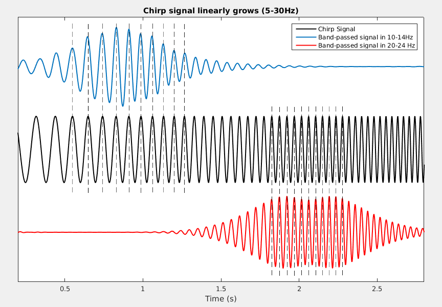
Function: brainstorm3/toolbox/math/bst_bandpass_hfilter.m
External call: process_bandpass('Compute', x, Fs, HighPass, LowPass, 'bst-hfilter', isMirror, isRelax)
Code:
1 function [x, FiltSpec, Messages] = bst_bandpass_hfilter(x, Fs, HighPass, LowPass, isMirror, isRelax, Function, TranBand, Method) 2 % BST_BANDPASS_HFILTER Linear phase FIR bandpass filter. 3 % 4 % USAGE: [x, FiltSpec, Messages] = bst_bandpass_hfilter(x, Fs, HighPass, LowPass, isMirror=0, isRelax=0, Function=[detect], TranBand=[], Method='bst-hfilter-2019') 5 % [~, FiltSpec, Messages] = bst_bandpass_hfilter([], Fs, HighPass, LowPass, isMirror=0, isRelax=0, Function=[detect], TranBand=[], Method='bst-hfilter-2019') 6 % x = bst_bandpass_hfilter(x, Fs, FiltSpec) 7 % 8 % DESCRIPTION: 9 % - A linear phase FIR filter is created. 10 % - Function "kaiserord" and "kaiser" are used to set the necessary order for fir1. 11 % - The transition band can be modified by user. 12 % - Requires Signal Processing Toolbox for the following functions: 13 % kaiserord, kaiser, fir1, fftfilt. If not, using Octave-based alternatives. 14 % 15 % INPUT: 16 % - x : [nChannels,nTime] input signal (empty to only get the filter specs) 17 % - Fs : Sampling frequency 18 % - HighPass : Frequency below this value are filtered in Hz (set to 0 for low-pass filter only) 19 % - LowPass : Frequency above this value are filtered in Hz (set to 0 for high-pass filter only) 20 % - isMirror : isMirror (default = 0 no mirroring) 21 % - isRelax : Change ripple and attenuation coefficients (default=0 no relaxation) 22 % - Function : 'fftfilt', filtering in frequency domain (default) 23 % 'filter', filtering in time domain 24 % If not specified, detects automatically the fastest option based on the filter order 25 % - TranBand : Width of the transition band in Hz 26 % - Method : Version of the filter (2019/2016-18) 27 % 28 % OUTPUT: 29 % - x : Filtered signals 30 % - FiltSpec : Filter specifications (coefficients, length, ...) 31 % - Messages : Warning messages, if any 32 33 % @============================================================================= 34 % This function is part of the Brainstorm software: 35 % https://neuroimage.usc.edu/brainstorm 36 % 37 % Copyright (c) University of Southern California & McGill University 38 % This software is distributed under the terms of the GNU General Public License 39 % as published by the Free Software Foundation. Further details on the GPLv3 40 % license can be found at http://www.gnu.org/copyleft/gpl.html. 41 % 42 % FOR RESEARCH PURPOSES ONLY. THE SOFTWARE IS PROVIDED "AS IS," AND THE 43 % UNIVERSITY OF SOUTHERN CALIFORNIA AND ITS COLLABORATORS DO NOT MAKE ANY 44 % WARRANTY, EXPRESS OR IMPLIED, INCLUDING BUT NOT LIMITED TO WARRANTIES OF 45 % MERCHANTABILITY AND FITNESS FOR A PARTICULAR PURPOSE, NOR DO THEY ASSUME ANY 46 % LIABILITY OR RESPONSIBILITY FOR THE USE OF THIS SOFTWARE. 47 % 48 % For more information type "brainstorm license" at command prompt. 49 % =============================================================================@ 50 % 51 % Authors: Hossein Shahabi, Francois Tadel, John Mosher, Richard Leahy, 52 % 2016-2019 53 54 55 %% ===== PARSE INPUTS ===== 56 % Filter is already computed 57 if (nargin == 3) 58 FiltSpec = HighPass; 59 % Default filter options 60 else 61 if (nargin < 9) || isempty(Method) 62 Method = 'bst-hfilter-2019' ; 63 end 64 if (nargin < 8) || isempty(TranBand) 65 TranBand = []; 66 end 67 if (nargin < 7) || isempty(Function) 68 Function = []; % Auto-detection based on the filter order later in the code 69 end 70 if (nargin < 6) || isempty(isRelax) 71 isRelax = 0; 72 end 73 if (nargin < 5) || isempty(isMirror) 74 isMirror = 0; 75 end 76 FiltSpec = []; 77 end 78 Messages = []; 79 80 81 %% ===== CREATE FILTER ===== 82 if isempty(FiltSpec) 83 % ===== FILTER SPECIFICATIONS ===== 84 Nyquist = Fs/2; 85 % High-pass filter 86 if ~isempty(HighPass) && (HighPass ~= 0) 87 f_highpass = HighPass / Nyquist; % Change frequency from Hz to normalized scale (0-1) 88 switch Method 89 case 'bst-hfilter-2019' 90 if isempty(TranBand) || TranBand==0 91 if (HighPass <= 5) 92 LwTranBand = .5 ; %Hz 93 else 94 LwTranBand = 1 ; %Hz 95 end 96 f_highstop = f_highpass - LwTranBand/Nyquist; 97 else 98 f_highstop = max(0, HighPass - TranBand) / Nyquist; 99 % f_highstop = max(0.2, HighPass - TranBand) / Nyquist; 100 TranBand = (f_highpass - f_highstop)*Nyquist ; % Adjusted Transition band 101 end 102 case 'bst-hfilter-2016' 103 % Default transition band 104 if (HighPass <= 5) % Relax the transition band if HighPass<5 Hz 105 f_highstop = .5 * f_highpass; 106 else 107 f_highstop = .85 * f_highpass; 108 end 109 end 110 else 111 f_highpass = 0; 112 f_highstop = 0; 113 LwTranBand = 1 ; 114 end 115 % Low-pass filter 116 if ~isempty(LowPass) && (LowPass ~= 0) 117 f_lowpass = LowPass / Nyquist; 118 switch Method 119 case 'bst-hfilter-2019' 120 if isempty(TranBand) || TranBand==0 121 UpTranBand = 1 ; 122 UpTranBand = min(UpTranBand,LwTranBand) ; 123 f_lowstop = f_lowpass + UpTranBand/Nyquist; 124 else 125 f_lowstop = f_lowpass + TranBand/Nyquist; 126 end 127 case 'bst-hfilter-2016' 128 % Default transition band 129 if f_highpass==0 % If this is a low-pass filter 130 f_lowstop = 1.05 * f_lowpass; 131 else 132 f_lowstop = 1.15 * f_lowpass; 133 end 134 end 135 else 136 f_lowpass = 0; 137 f_lowstop = 0; 138 end 139 % If both high-pass and low-pass are zero 140 if (f_highpass == 0) && (f_lowpass == 0) 141 Messages = ['No frequency band in input.' 10]; 142 return; 143 % Input frequencies are too high 144 elseif (f_highpass >= 1) || (f_lowpass >= 1) 145 Messages = sprintf('Cannot filter above %dHz.\n', Nyquist); 146 return; 147 end 148 % Transition parameters 149 if isRelax 150 Ripple = 10^(-2); 151 Atten = 10^(-2); % Equals 40db 152 else 153 Ripple = 10^(-3); % pass band ripple 154 Atten = 10^(-3); % Equals 60db 155 end 156 157 % ===== DESIGN FILTER ===== 158 % Build the general case first 159 fcuts = [f_highstop, f_highpass, f_lowpass, f_lowstop]; 160 mags = [0 1 0]; % filter magnitudes 161 devs = [Atten Ripple Atten]; % deviations 162 % Now adjust for desired properties 163 fcuts = max(0,fcuts); % Can't go below zero 164 fcuts = min(1-eps, fcuts); % Can't go above or equal to 1 165 166 % We have implicitly created a bandpass, but now adjust for desired filter 167 if (f_lowpass == 0) % User didn't want a lowpass 168 fcuts(3:4) = []; 169 mags(3) = []; 170 devs(3) = []; 171 end 172 if (f_highpass == 0) % User didn't want a highpass 173 fcuts(1:2) = []; 174 mags(1) = []; 175 devs(1) = []; 176 end 177 178 % Generate FIR filter 179 % Using Matlab's Signal Processing toolbox 180 if bst_get('UseSigProcToolbox') 181 [n,Wn,beta,ftype] = kaiserord(fcuts, mags, devs, 2); 182 n = n + rem(n,2); % ensure even order 183 b = fir1(n, Wn, ftype, kaiser(n+1,beta), 'noscale'); 184 % Using Octave-based functions 185 else 186 [n,Wn,beta,ftype] = oc_kaiserord(fcuts, mags, devs, 2); 187 n = n + rem(n,2); % ensure even order 188 b = oc_fir1(n, Wn, ftype, oc_kaiser(n+1,beta), 'noscale'); 189 end 190 191 % Filtering function: Detect the fastest option, if not explicitely defined 192 if isempty(Function) 193 % The filter() function is a bit faster for low-order filters, but much slower for high-order filters 194 if (n > 800) % Empirical threshold 195 Function = 'fftfilt'; 196 else 197 Function = 'filter'; 198 end 199 end 200 201 % Compute the cumulative energy of the impulse response 202 E = b((n/2)+1:end) .^ 2 ; 203 E = cumsum(E) ; 204 E = E ./ max(E) ; 205 % Compute the effective transient: Number of samples necessary for having 99% of the impulse response energy 206 [tmp, iE99] = min(abs(E - 0.99)) ; 207 208 % Output structure 209 FiltSpec.b = b; 210 FiltSpec.a = 1; 211 FiltSpec.order = n; 212 FiltSpec.transient = iE99 / Fs ; % Start up and end transients in seconds (Effective) 213 % FiltSpec.transient_full = n / (2*Fs) ; % Start up and end transients in seconds (Actual) 214 FiltSpec.f_highpass = f_highpass; 215 FiltSpec.f_lowpass = f_lowpass; 216 FiltSpec.fcuts = fcuts * Nyquist ; % Stop and pass bands in Hz (instead of normalized) 217 FiltSpec.function = Function; 218 FiltSpec.mirror = isMirror; 219 % If empty input: just return the filter specs 220 if isempty(x) 221 return; 222 end 223 end 224 225 %% ===== FILTER SIGNALS ===== 226 % Transpose signal: [time,channels] 227 [nChan, nTime] = size(x); 228 % Half of filter length 229 M = FiltSpec.order / 2; 230 % If filter length > 10% of data length 231 edgePercent = 2*FiltSpec.transient / (nTime / Fs); 232 if (edgePercent > 0.1) 233 Messages = [Messages, sprintf('Start up and end transients (%.2fs) represent %.1f%% of your data.\n', 2*FiltSpec.transient, 100*edgePercent)]; 234 end 235 236 % Remove the mean of the data before filtering 237 xmean = mean(x,2); 238 x = bst_bsxfun(@minus, x, xmean); 239 240 % Mirroring requires the data to be longer than the filter 241 if (FiltSpec.mirror) && (nTime < M) 242 Messages = [Messages, 'Warning: Data is too short for mirroring. Option is ignored...' 10]; 243 FiltSpec.mirror = 0; 244 end 245 % Mirror signals 246 if (FiltSpec.mirror) 247 x = [fliplr(x(:,1:M)), x, fliplr(x(:,end-M+1:end))]; 248 % Zero-padding 249 else 250 x = [zeros(nChan,M), x, zeros(nChan,M)] ; 251 end 252 253 % Filter signals 254 switch (FiltSpec.function) 255 case 'fftfilt' 256 if bst_get('UseSigProcToolbox') 257 x = fftfilt(FiltSpec.b, x')'; 258 else 259 x = oc_fftfilt(FiltSpec.b, x')'; 260 end 261 case 'filter' 262 x = filter(FiltSpec.b, FiltSpec.a, x, [], 2); 263 end 264 265 % Remove extra data 266 x = x(:,2*M+1:end); 267 % Restore the mean of the signal (only if there is no high-pass filter) 268 if (FiltSpec.f_highpass == 0) 269 x = bst_bsxfun(@plus, x, xmean); 270 end
Filter specifications: Notch
Description: 2nd order IIR notch filter with zero-phase lag (implemented with filtfilt).
Reference: Mitra, Sanjit Kumar, and Yonghong Kuo. Digital signal processing: a computer-based approach. Vol. 2. New York: McGraw-Hill, 2006. MatlabCentral #292960
Edge effects: It is computed based on the 99% energy of the estimated impulse response.
Function: brainstorm3/toolbox/process/functions/process_notch.m
External call: [x, FiltSpec, Messages] = Compute(x, sfreq, FreqList, Method, bandWidth)
Filter specifications: Band-stop
Description: 4th order Butterworth IIR filter with zero-phase lag (implemented with filtfilt)
Reference: FieldTrip: x = ft_preproc_bandstopfilter(x, sfreq, FreqBand, [], 'but', 'twopass')
Edge effects It is computed based on the 99% energy of the estimated impulse response.
Function: brainstorm3/toolbox/process/functions/process_bandstop.m
External call: x = process_bandstop('Compute', x, sfreq, FreqList, FreqWidth)
On the hard drive
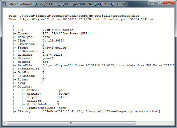
The names of the files generated by the process "Power spectrum density" start with the tag timefreq_psd, they share the same structure as all the files that include a frequency dimension.
To explore the contents of a PSD file created in this tutorial, right-click on it and use the popup menus
File > View file contents or File > Export to Matlab.
Structure of the time-frequency files: timefreq_psd_*.mat
TF: [Nsignals x Ntime x Nfreq] Stores the spectrum information. Nsignals is the number of channels that were selected with the option "MEG" in the PSD process. Nfreq is the number of frequency bins. There is no time dimension (Ntime = 1).
Comment: String used to represent the file in the database explorer.
Time: Window of time over which the file was estimated.
TimeBands: Defined only when you select the option "Group in time bands".
Always empty for the PSD files because there is no time dimension.Freqs: [1 x Nfreq] List of frequencies for which the power spectrum was estimated (in Hz).
RefRowNames: Only used for connectivity results.
RowNames: [Nsignals x 1] Describes the rows of the TF matrix (first dimension). Here it corresponds to the name of the MEG sensors, in the same order as is the .TF field.
Measure: Function currently applied to the FFT coefficients {power, none, magnitude, log, other}
Method: Function that was used to produce this file {psd, hilbert, morlet, corr, cohere, ...}
DataFile: File from which this file was calculated = Parent file in the database explorer.
DataType: Type of file from which this file was calculated (file type of .DataFile).
- 'data' = Recordings
- 'cluster' = Recordings grouped by clusters of sensors
- 'results' = Source activations
- 'scouts' = Time series associated with a region of interest
SurfaceFile / GridLoc / GridAtlas / Atlas: Used only when the input file was a source file.
Leff: Effective number of averages = Number of input files averaged to produce this file.
Options: Most relevant options that were passed to the function bst_timefreq.
History: Describes all the operations that were performed with Brainstorm on this file. To get a better view of this piece of information, use the menu File > View file history.
Useful functions
in_bst_timefreq(PsdFile): Read a PSD or time-frequency file.
in_bst(FileName): Read any Brainstorm file.
bst_process('LoadInputFile', FileName, Target): The most high-level function for reading Brainstorm files. "Target" is a string with the list of sensor names or types to load (field RowNames).
bst_psd(F, sfreq, WinLength, WinOverlap): Computation of the Welch's power spectrum density.
Additional documentation
Forum discussions

