Fitting dipoles with FieldTrip

Authors: Jeremy Moreau

This tutorial introduces dipole fitting and visualisation in Brainstorm. You will need to have completed the introductory tutorials up to "Tutorial 16: Average response" before undertaking this tutorial. This tutorial explains how to fit dipoles to time series within Brainstorm. If you already have computed dipole fits using CTF DipoleFit or Neuromag XFit and would like to import them in Brainstorm, see this tutorial.

Warning: This function does not work properly with FieldTrip versions released between 2015-10-05 and 2016-01-15. If you are using a version released around this time, update FieldTrip first.

Fitting dipoles using process FieldTrip: ft_dipolefitting

This process wraps the FieldTrip function ft_dipolefitting. For background information on the implementation of the dipole modelling see the FieldTrip dipole fitting tutorial or watch this video. Note that in order to use this process you will need to have FieldTrip installed and added to your Matlab path.

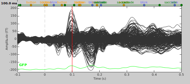
We will be fitting dipoles to the auditory ERFs computed in "Tutorial 16: Average response". In a first step, we will fit a single dipole to the peak of the M100 ERF component.

• Open the protocol TutorialIntroduction and switch to the "functional data" view.

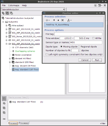
• Expand the run 02 folder (not the Raw link), and drag the average time series "Avg: standard" into the Process1 box.

• Click on "Run" and select the process Sources -> FieldTrip: ft_dipolefitting.

• Enter M100 in the "File tag" field, 100 - 100 in the "Time window" fields, and leave all other options as they are. Press "Run" and wait (you may want to look at the Matlab console to see the progress).

• Once the process is done computing a new dipole file will appear in your database under the average time series on which it was computed. Before continuing to visualising the dipoles, let's compute a second dipole around the M50 component. This time we'll fit a moving dipole over a 20ms time window around the peak of the M50.

Visualising dipole files

• Double click the M100 dipole file generated in the previous section. This will open up the 3D MRI viewer. For more information on usage and basic options of the 3D MRI viewer refer to the "MRI in 3D" subsection of Tutorial 3.

• Dipoles are coloured according to time by default, but since we've fit a dipole to a single time point in this case this option is not very useful. Under the Dipoles tab of the main Brainstorm window look for the "Color dipoles according to" subsection, and select "Goodness of fit". Larger values represent a better fit, but note that "goodness of fit" values computed using the "FieldTrip: ft_dipolefitting" process are not equivalent to those of imported CTF DipoleFit or Neuromag XFit dipoles. FieldTrip's ft_dipolefitting function computes residual variance as its measure of goodness of fit. In Brainstorm, we plot the explained variance (i.e. 1 - residual variance).

• Now close the current 3D MRI viewer, and double click the M50 dipole file. You'll now see a series of dipoles plotted on the 3d MRI viewer.

• Switch between the "Time" and "Goodness of fit" options to get an idea of when the best fit occurs. You can also select the "Show max goodness of fit" option to display only the dipole with the best fit or move the "Goodness" slider to hide all dipoles with a goodness value under a selected threshold.

Merging dipole files

You may sometimes want to visualise multiple sets of dipoles together on the same MRI viewer. For instance, you may have fit dipoles to a series of individual epileptic spikes, and would like to see whether the dipoles form a cluster. In the context of this tutorial, we are going to merge the M50 dipole file with the M100 dipole file, so that we can see where they localise relative to each other.

• In the main Brainstorm window, select the dipole files to merge (hold down shift and click on each dipole file). Then right-click on any one of the dipole files and select "Merge dipoles". A new dipole file will be created in your database called "Merge: 2 files". Double click it to display.

• In addition to the "Time" and "Goodness of fit" colouring options, you'll find that the "Group" option is useful when viewing merged dipole files. This option colours dipoles from each of the original dipole files in a different colour.

FieldTrip: ft_dipolefitting process options

File tag: Text string that will be added at the end of the comment field of the dipole file.

Time window: Time window over which to run the dipole fit. If you want to fit a dipole to a single time point enter the same time value in the start and end field.

Sensor type or names: Type of sensor (e.g. MEG, EEG) or comma separated list of sensor names (e.g. MLF42) to use in the dipole fit. It is not currently possible to select multiple sensor types at once (e.g. both MEG and EEG).

Dipole type: For each time sample within the selected time window, the moving dipole option fits a dipole with a different position and orientation, whereas the regional dipole option fits a dipole with a different orientation but always the same position.

Number of dipoles to fit: The number of dipoles that will be fit at each time point.

Left-right symmetry constraint: Selecting this option imposes a left-right symmetry constraint when fitting two dipoles. You may want to use this when you have a reason to believe that bilateral activation may be occuring (e.g. because you are delivering a stimulus bilaterally).

---