Fitting dipoles with FieldTrip
Authors: Jeremy Moreau, Francois Tadel
This tutorial introduces dipole fitting and visualization in Brainstorm. You will need to have completed the introduction tutorials up to "Tutorial 16: Average response" before undertaking this tutorial. This tutorial explains how to fit dipoles to time series within Brainstorm. If you already have computed dipole fits using CTF DipoleFit or Neuromag XFit and would like to import them in Brainstorm, see this tutorial.
Contents
Requirements
This process wraps the FieldTrip function ft_dipolefitting. You can install FieldTrip manually or as a Brainstorm plugin, as exaplined in the Plugins tutorial.
For background information on the implementation of the dipole modeling see the FieldTrip dipole fitting tutorial or watch this video.
This process requires a pre-computed spherical head model. As the forward solution for the dipoles need to be recomputed at each iteration during the fitting procedure, only the simplest (i.e. spherical) models are currently supported (so OpenMEEG models will not work).
Process FieldTrip: ft_dipolefitting
Open the protocol TutorialIntroduction and switch to the "functional data" view.
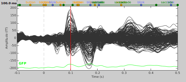
We will be fitting dipoles to the auditory ERFs computed in the tutorial Average response. In a first step, we will fit a single dipole to the peak of the M100 ERF component (100ms).
- Expand the imported run01 and drag the average time series "Avg: standard" into the Process1 box.
Run process Sources > FieldTrip: ft_dipolefitting: Time window=[100,100]ms, Sensors=MEG
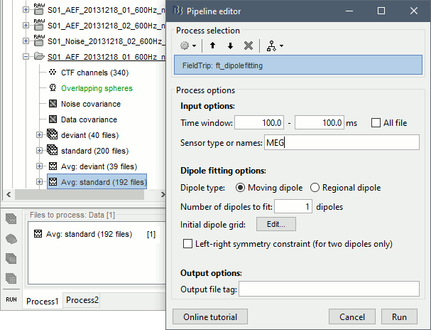
- Press "Run" and wait. Check the Matlab console for the progress.
Once the process is done computing a new dipole file will appear in your database under the average time series on which it was computed. Before continuing to visualizing the dipoles, let's compute a second dipole around the M50 component. This time we'll fit a moving dipole over a 20ms time window around the peak of the M50.
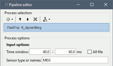
Process options
Time window: Time window over which to run the dipole fit. If you want to fit a dipole to a single time point enter the same time value in the start and end field.
Sensor type or names: Type of sensor (e.g. MEG, EEG) or comma separated list of sensor names (e.g. MLF42) to use in the dipole fit. It is not currently possible to select multiple sensor types at once (e.g. both MEG and EEG).
Dipole type: For each time sample within the selected time window, the moving dipole option fits a dipole with a different position and orientation, whereas the regional dipole option fits a dipole with a different orientation but always the same position.
Number of dipoles to fit: The number of dipoles that will be fit at each time point.
Initial dipole grid: When fitting a single dipole, the dipole fitting algorithm starts with estimating the goodness of fit of a fixed grid of dipoles, then takes the best fitting one and refines it with an iterative dipole fitting algorithm. When fitting multiple dipoles, this initial grid search is disabled because it is not supported by the function ft_dipolefitting.
Left-right symmetry constraint: Selecting this option imposes a left-right symmetry constraint when fitting two dipoles. You may want to use this when you have a reason to believe that bilateral activation may be occuring (e.g. because you are delivering a stimulus bilaterally).
File tag: Text string that will be added at the end of the comment field of the dipole file.
Visualizing dipole files
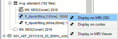
Double click the M100 dipole file generated in the previous section. This will open up the 3D MRI viewer. For more information on usage and basic options of the 3D MRI viewer, see this tutorial.
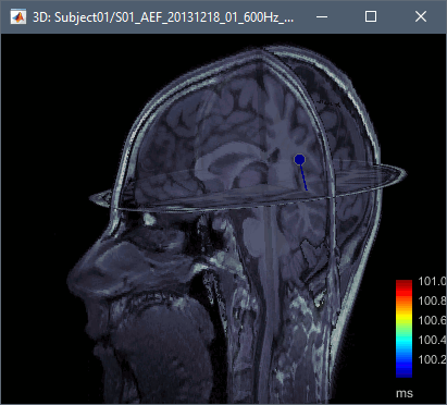
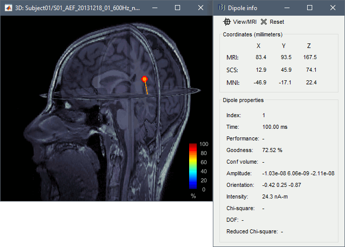
Dipoles are coloured according to time by default, but since we've fit a dipole to a single time point in this case this option is not very useful. Under the Dipoles tab of the main Brainstorm window look for the "Color dipoles according to" subsection, and select "Goodness of fit". Larger values represent a better fit, but note that "goodness of fit" values computed using the "FieldTrip: ft_dipolefitting" process are not equivalent to those of imported CTF DipoleFit or Neuromag XFit dipoles. FieldTrip's ft_dipolefitting function computes residual variance as its measure of goodness of fit. In Brainstorm, we plot the explained variance (i.e. 1 - residual variance).
Click on the dipole to get detailed information about its position, amplitude and significance. This single dipole localizes correctly the left primary auditory cortex, but it shows a goodness of fit of ~70%, which is a relatively poor performance for an average response with such a high SNR. This is due to the fact that there are multiple simultaneous sources (more details in the following section).
- Now close the current 3D MRI viewer, and double click the other dipole file (40-60ms). You'll now see a series of dipoles plotted on the 3d MRI viewer.
Switch between the "Time" and "Goodness of fit" options to get an idea of when the best fit occurs. You can also select the "Show max goodness of fit" option to display only the dipole with the best fit or move the "Goodness" slider to hide all dipoles with a goodness value under a selected threshold.
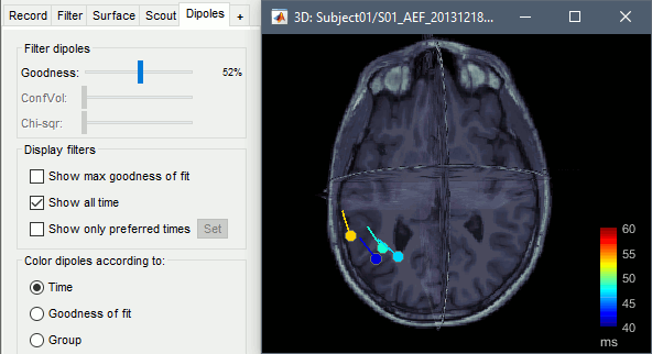
- The position of these dipoles could make sense, but the associated measures of goodness of fit are very low (around 50%). A single dipole can explain the activity of only one source at a time, and would fail at explaining correctly the activity of simultaneous sources (e.g. left and right auditory cortex).
Multiple dipoles
In the two examples above, we fitted one single dipole at each time point. This approach is expected to work well if we assume that there is one active source only at each time point. This is not the case here as we expect a bilateral auditory response to this binaural sitmulus. We obtained results that look meaningful (dipoles close to the auditory regions) because the response we recorded is stronger on the left side, but with a truly symmetrical response we could have obtained a dipole in the center of the head. This approach is globally wrong for multiple sources.
If you expect to observe two sources of activity simultaneously, then you need to either fit two dipoles at the same time, or to use a distributed source model. However, there are difficult methodological problems that come with multiple dipole fitting: Do you fit first a dipole and then fit a second one to the residuals? Do you try to optimize the two dipoles at once? Obtaining correct results usually requires an accurate manual initialization of the dipoles parameters, and a lot of user supervision over the process.
Let's see what happens if we ask the FieldTrip function to fit two dipoles, in order to explain the activity of the left and right auditory cortices simultaneously.
Run the process Sources > FieldTrip: ft_dipolefitting: Time window=[40,60]ms, Sensors=MEG, Number of dipoles to fit: 2, Left-right symmetry=No
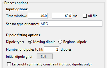
You can uncheck the option "Show all times" and then navigate in time between 40ms and 60ms post-stimulus, in order to observe the pairs of dipoles that were fitted at each time point.
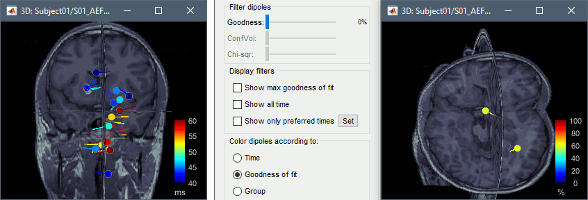
The result is not very convincing, all the dipoles are too close to the mid-sagittal plane. The convergence of this algorithm depends a lot on the initialization of the two dipoles. When fitting a single dipole, the FieldTrip algorithm starts by computing the performance of a fixed grid of dipoles and initializes the non-linear fit loop with the most significant dipole on this grid. This option is not supported by ft_dipolefitting for multiple dipoles. The two dipoles are then initialized to the center of the head (0,0,0) and the fitting algorithm doesn't converge correctly.
- It is possible to obtain much better results by initializing the position and orientation of the two dipoles in a more realistic way, but it requires a lot of manual steps and may produce very different results depending on who places the dipoles. This is not an approach we promote in Brainstorm.
One additional option exist in ft_dipolefitting, to constrain the fitting to two symmertrical dipoles. In this case, the initial grid search is available and the algorithm convergence is a lot better. Run the same process again, with the option "Left-right symmetry" selected.
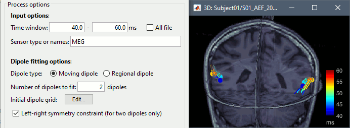
- These results look a lot better, but if we give a closer look at the location of the dipoles, we can see that they don't align very well with the auditory cortex on either side. In general, it is very unlikely that two corresponding anatomical regions are strictly symmetrical left-right. This option is a patch to the multiple dipole fitting, but not exactly a good solution either.
Conclusion
Single dipole fitting is great to identify focal sources in the brain, when there are no other co-occurring events. It can be particularly convenient to localize the focus area of epileptic spikes, as shown in tutorial EEG and epilepsy: Dipole fitting.
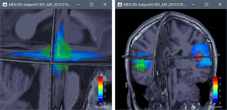
When more than one region of the brain might be involved, we recommend using distributed source models (surface or volume), that are much better able to represent multiple sources simultaneously. Screen captures below from the tutorial : Volume source estimation.
Merging dipole files
You may sometimes want to visualize multiple sets of dipoles together on the same MRI viewer. For instance, you may have fit dipoles to a series of individual epileptic spikes, and would like to see whether the dipoles form a cluster. In the context of this tutorial, we are going to merge the M50 dipole file with the M100 dipole file, so that we can see where they localise relative to each other.
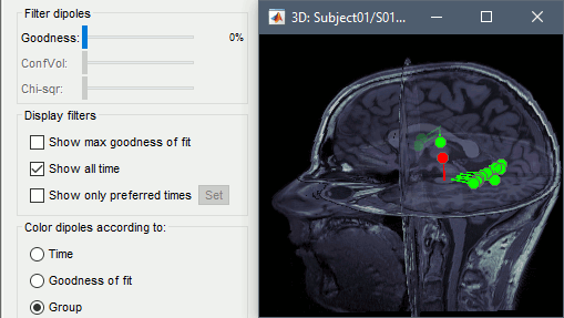
- In the main Brainstorm window, select the dipole files to merge (hold down shift and click on each dipole file). Then right-click on any one of the dipole files and select "Merge dipoles". A new dipole file will be created in your database called "Merge: 2 files". Double click it to display.
In addition to the "Time" and "Goodness of fit" colouring options, you'll find that the "Group" option is useful when viewing merged dipole files. This option colours dipoles from each of the original dipole files in a different colour.
Additional documentation
Brainstorm tutorial: EEG and epilepsy: Dipole fitting
Brainstorm tutorial: Dipoles: Scanning and displaying
Brainstorm tutorial: MEG current phantom (CTF)
FieldTrip reference: ft_dipolefitting
FieldTrip tutorial: Dipole fitting of combined MEG/EEG data

