Best: Brain Entropy in space and time
[TUTORIAL UNDER DEVELOPMENT]
A first release of the BEst v2.6 package is for now distributed within this version of Brainstorm.
Using this version of Brainstorm, a prompt will ask you to proceed with the installation of the Package at the first launch of Brainentropy MEM source localization.
The inclusion of the package within the standard distribution of Brainstorm is planned for the end of September 2014.
Authors: Zerouali Y, Lacourse K, Chowdhury R, Hedrich T, Lina JM, Grova C.
Are you interested in estimating the spatial extent of EEG/MEG sources?
Are you interested in localizing oscillatory patterns?
Are you interested in localizing synchronous cortical sources?

This tutorial introduces the toolbox BEst – "Brain Entropy in space and time" that implements several EEG/MEG source localization techniques within the “Maximum Entropy on the Mean (MEM)” framework. These methods are particularly dedicated to estimate accurately the source of EEG/MEG generators together with their spatial extent along the cortical surface. Assessing the spatial extent of the sources might be very important in some application context, and notably when localizing spontaneous epileptic discharges. We also proposed two other extensions of the MEM framework within the time frequency domain dedicated to localize oscillatory patterns in specific frequency bands and synchronous sources.
Contents
Introduction
BEst toolbox is the result of a collaborative work between two research teams:
|
LATIS Lab directed by Dr. Jean Marc Lina, Prof. in Electrical Engineering Dpt at Ecole de Technologie Supérieure, Montréal. Main students involved: Younes Zerouali and Karine Lacourse |
|
Multimodal Functional Imaging Lab directed by Dr. Christophe Grova, Prof. in Biomedical Engineering Dpt and Neurology and Neurosurgery Dpt, McGill University. Main students involved: Rasheda Chowdhury and Tanguy Hedrich |
The package proposes three methods:
cMEM: Standard MEM with stable clustering source localization in the time-domain. The originality of this method is its ability to recover to the spatial extent of the underlying sources. To do so, the solution is estimated using a unique, but optimal, parcelization of the cortex as spatial prior. These parcels are estimated assuming brain activity to be spatially stable. (Chowdhury et al. Plos One 2013)
wMEM: wavelet based MEM dedicated to perform source localization of oscillatory patterns in the time-frequency domain. The data and the solution are expressed in a discrete wavelet expansion. The spatial prior is a parcelization of the cortex specific to each time-frequency piece of the data (Lina et al. IEEE TBME 2012).
rMEM: ridge MEM dedicated to localize cortical sources exhibiting synchrony. Continuous complex-valued wavelet analysis of the data allows detection data segments exhibiting synchrony between sensors. rMEM consists in localizing the generators of these detected synchrony patterns (Zerouali et al. IEEE TBME 2013).
See below for more information on the BEst license and the associated publications.
Principle of the “Maximum Entropy on the Mean”
The MEM solver relies on a probabilistic (Bayesian) approach where inference on the current source intensities is estimated from the informational content in the data (notion of maximum of entropy): “The maximum entropy distribution is uniquely determined as the one which is maximally noncommittal with regard to missing information” (E.T. Jaynes, Information and statistical mechanics, Phys. Rev. 106(4), 1957). The first applications of MEM in electromagnetic source localization were proposed by Clarke and Janday (The solution of biomagnetic inverse problem by maximum statistical entropy, Inv. Problem 5, 1989). A concomitant work entitled “if realistic neurophysiological constraints are imposed, then maximum entropy is the most probable solution of the EEG inverse problem” (Inv. Problem 6, 1990) was published by Rice.
The main contribution of our group consists in the prior model that we consider within the MEM regularization framework. It started with the idea of describing brain activity as being organized by cortical parcels, each parcel having the possibility of being active or not, whereas MEM offers the possibility to estimate a contrast of current density within each active parcel. This idea was first introduced within the classical MEM framework by Amblard et al. (Biomagnetic source detection by Maximum Entropy and Graphical Models, IEEE TBME, 2004), using notably data-driven approaches to estimate the cortical parcels (Lapalme et al., Data-driven parceling and entropic inference in MEG, NeuroImage, 2006). The use of such a spatial model within the MEM framework is the key idea allowing MEM to be sensitive to the spatial extent of the sources along the cortical surface (Grova et al. Evaluation of EEG localization methods using realistic simulations of interictal spikes. Neuroimage 2006). The most recent development consists in the extension of MEM within the time frequency domain in order to localize oscillatory and synchronous generators.
Best toolbox offers three different kind of information to be localized on the cortex: generators with time series stable within parcels; generators of oscillatory patterns and generators of synchrony.
MEM: dataset and preliminary steps
- This tutorial illustrates the use of cMEM, wMEM and rMEM on MEG averaged responses (98 trials) to a Median Nerve electrical Stimulation (MNS). The tutorial can be obtained in two ways: either you download the Brainstorm dataset used in the introductory tutorials, or you download a protocol where all the preprocessed has been already performed.
Brainstorm database
- This dataset corresponds to the standard MNS dataset provided in Brainstorm:
sample_raw.zip in http://neuroimage.usc.edu/bst/download.php.
- To use this dataset, following steps should be done to prepare the data for localization:
If this is your first time using Brainstorm, you will have to define a folder to store your Brainstorm database (cf. Brainstorm starting tutorials for further details) .
- Download and unzip the sample_raw.zip file.
- In brainstorm, create a new protocol and a new subject
In the anatomy view, right-click on the subject > Import anatomy folder, select the file format "FreeSurfer folder" and select the folder "sample_raw/Anatomy".
Set the number of vertices of the cortex surface at 10000. Too many number of vertices will make the process of parcellization time-consuming
- The MRI coordinates of the fiducials are:
- NAS: x=127, y=211, z=126
- LPA: x=58, y=132, z=118
- RPA: x=197, y=133, z=114
- AC: x=128, y=138, z=158
- PC: x=128, y=112, z=158
- IH: x=129, y=112, z=227 (anywhere on the midsagittal plane)
- Switch to “Functional data (sorted by subject)” view.
Right click on the Subject01> Import MEG/EEG
- File format: "MEG/EEG: CTF .ds (*.meg4;*.res4)" (Select the full directory and click open)
- Choose the right hand MNS data (Epoch time: -1000 to +1000 ms; remove DC offset: All recordings; subsample to 600Hz; uncheck “Create a separate folder for each epoch type”), click Import
- Click Yes for sensor/anatomy registration.
- Bandpass filter the data from 0.3 to 70Hz using the process method.
- Average the 98 trials.
Switch to the “Anatomy” view of this protocol, right click on the Subject01> Generate BEM surfaces using the default parameters.
Switch to the “Functional data” view; right click on the Subject01> Compute head model.
- Select OPENMEEG BEM, click Ok
- Set the conductivity of the Brain layer to 0.33, click Ok. You can also choose to use a fully prepared database containing the averaged MEG response for right hand stimulation, MEG forward model and an example of cMEM localization of the whole MNS evoked response.
Right click on Subject01 > Noise covariance > No noise covariance. Unlike the other methods proposed in Brainstorm, MEM does not require prior calculation of a noise covariance matrix. This matrix can be estimated using a physiological baseline signal that can either be part of the data to be localized or a different piece of data. In some circumstances, the noise covariance matrix can be estimated from empty room data.
- To compute source localization, go to section "Launch BEst"
Preprocessed database
This database BEst_tutorial_median_nerve can be downloaded there. The objective of this tutorial is to guide you to produce these results. Note that unlike the other methods proposed in Brainstorm, MEM does not require prior calculation of a noise covariance matrix. To use the database directly, follow the following steps
Import the data in brainstorm by clicking: File > Load protocol > Load from zip file > browse the protocol and choose the zip file:
BST_sample_raw_Subject03 .zip
Launch BEst
- Go to the “Functional data (sorted by subject)” view
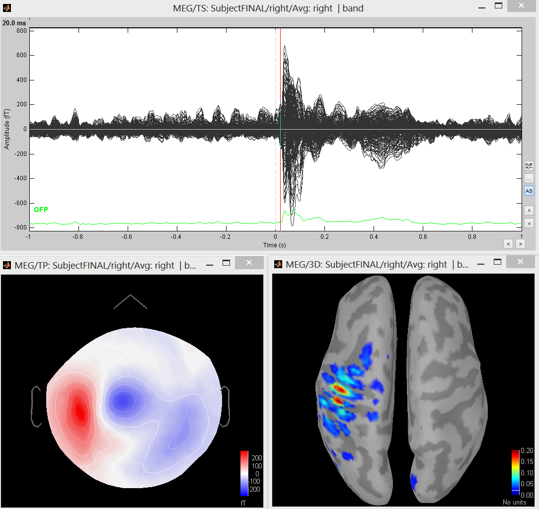
Right-click on the data average > Compute sources > Brain Entropy MEM > 'Ok' Note: The MEM option only appears in expert mode. Make sure it is toggled from the button at the bottom left. It is recommended that you customize the comment field so as to avoid confusion when performing multiple localizations for a given dataset.
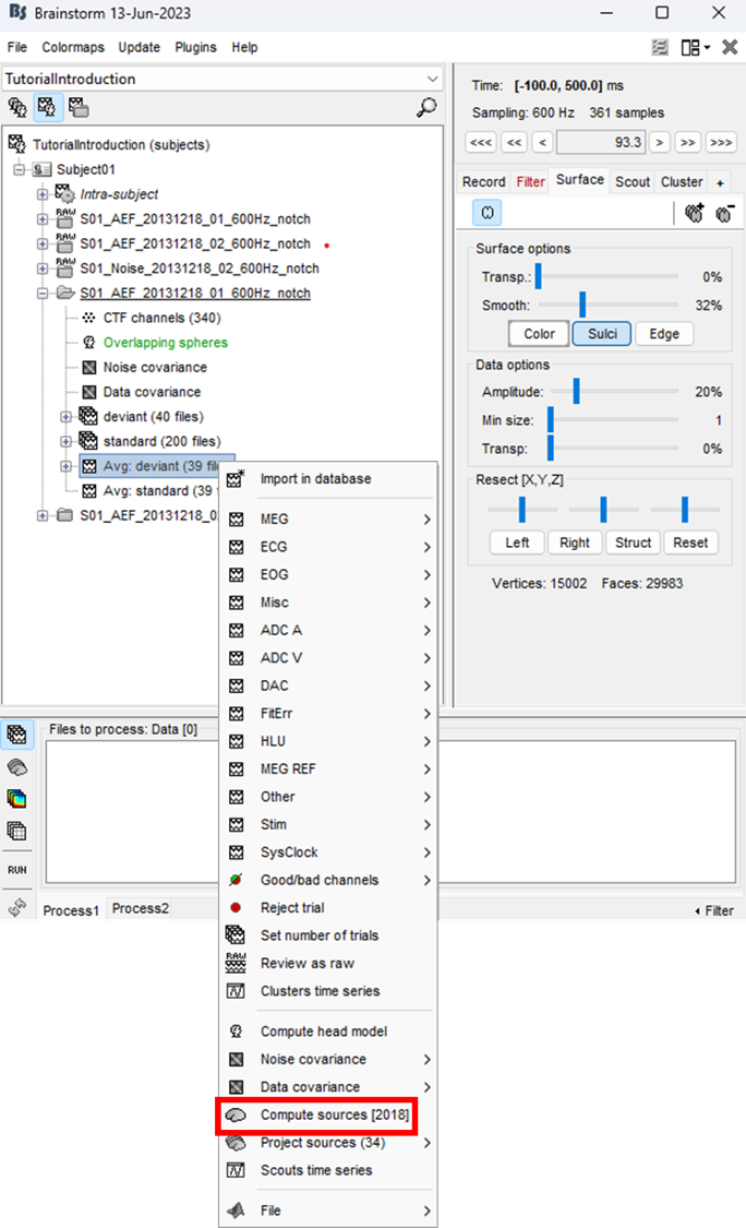
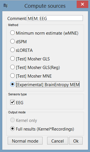
Select the MEM method (cMEM: time series representation, wMEM: time-scale representation, or rMEM: wavelet representation). Define the data time window and the baseline data while keeping other parameters at default values. Then hit 'Ok'.
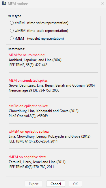
cMEM
You have clicked on cMEM. The panel then displays all the parameters associated with this method. Parameters are defined in two sets:
The left column proposes basic mandatory parameters
The right column proposes more subtle parameters, for more advanced users. To access this set of parameters, you need to click on the ‘expert’ option. The ‘OK’ will be then available once all mandatory parameters have been specified.
Using the BEst_tutorial_median_nerve, we propose the following first experiment:
1. Selection of a specific time window may be useful for long data epochs (default: localize whole data window).
Suggested time window for this dataset: 0.005 to 0.025 s.
This window is suggested to allow the localization of the first MNS response (N20, 20ms after the electrical stimulation). Note that cMEM requires an iterative estimation for each time sample. This is the reason why, cMEM localization along the whole MNS response is provided in the database, for illustration purposes during the workshop. Depending on your computer, you should be able to localize the whole time window with cMEM in about 10-15min.
2. Three choices are available for baseline definition. cMEM will consider such a baseline to estimate the noise covariance matrix in the sensor space.
○ Default: the panel looks for a dataset called 'baseline' within the same study as the data to be localized. When not found, this option is disabled.
○ Within data: the baseline is a time window to be selected within the recordings.
○ Import: the user can import baseline data from a file using brainstorm import tools. In any case, the user can define a time window for the baseline
Suggested baseline for this dataset:
within data, with interval -1 to -0.150 s.
3. Neighborhood order: this parameter defines the size of the parcels that will be constructed, independently in each time-frequency box. Here, we suggest using 4.
All other parameters can be kept with their default values:
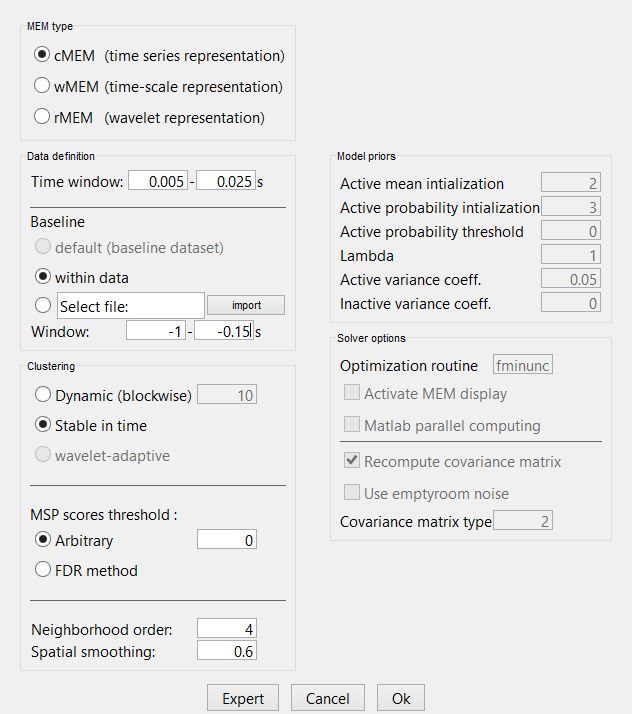
4. Hitting 'Ok' will launch cMEM estimation. At the end, a new results file appears in the database under the appropriate dataset. Simply double-click it to visualize.
We suggest to look at the sources around t = 0.020 s.
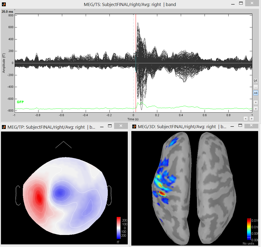
Other suggestion: run cMEM with a longer time window, i.e. 0.0 to 0.150 sec, to localize the whole MNS response.
Parameters of cMEM
● Clustering: Dynamic or stable in time
● MSP scores threshold: Arbitrary or FDR method
wMEM
You have clicked on wMEM. The panel then displays all the parameters associated with this method. Parameters are defined in two sets:
The left column proposes basic mandatory parameters.
The right column proposes more subtle parameters, for more advanced users. To access this set of parameters, you need to click on the ‘expert’ option. The ‘OK’ will be then available once all mandatory parameters have been specified.
Principle: The data is decomposed following a discrete multiresolution scheme using real Daubechies wavelets. The time-scale plane can then be threshold to keep only significant coefficients, up to a fraction of total signal power.
wMEM then localizes the sources associated to each wavelet coefficient of the time-scale plane, thus yielding an estimation of wavelet coefficients for each source. As we keep only significant oscillatory modes from the time-scale planes, this method efficiently targets the oscillating neural sources. Interestingly, the Daubechies wavelets have a stable inverse transform, which allows us to recover efficiently the time course associated to each source.
With the BEst_tutorial_median_nerve, we propose the following first experiment (similar to cMEM previous experiment)
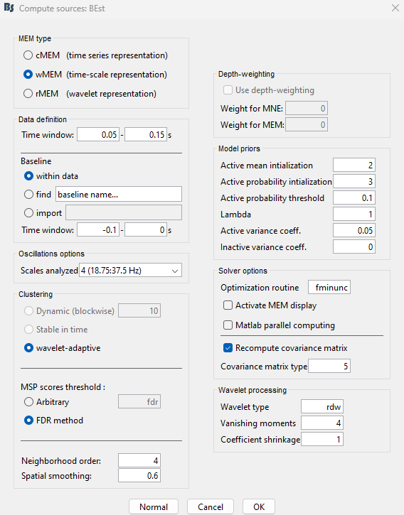
1. Selection of a specific time window may be useful to localize specific time-frequency components of the recordings (default: localize whole data window). Suggested time window for this dataset: 0.005 to 0.025 s.
2. Three choices are available for baseline definition.
Default: the panel looks for a dataset called 'baseline' within the same study as the data to be localized. When not found, this option is disabled. Within data: the baseline is a time window within the recordings. Import: the user can import baseline data from a file using brainstorm import tools. In all cases, the user can define a time window for the baseline Suggested baseline for this dataset: within data, with interval -1 to -0.150 s
3. Selection of scales to be localized. Suggested scale = 3 (corresponding to frequency band: 37 to 75 Hz). This is the highest frequency component of the peak at t = 20 ms.
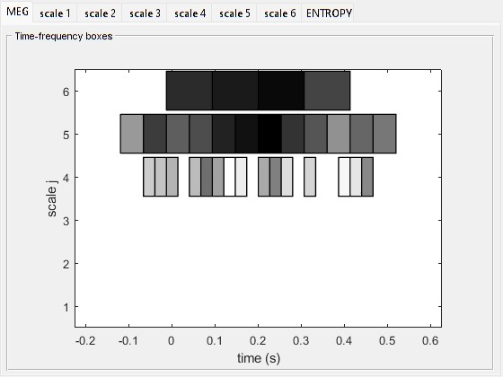
This figure, that you can get by selecting MEM display in the ‘expert parameters’ column, shows the global Multi-Resolution power (mean wavelet power over all MEG sensors). Each box corresponds to a wavelet at some scale (index j) and located in time. The scale ( j ) increases with the inverse of the frequency: the lower is j, the faster the local oscillation. The darker is a box, the more power is associated with it. As expected, the evoked response recruits high frequencies between 0 and 0.2 s. With the above scale selected (j = 3, frequency: 37-75 Hz), we pick only a piece of the oscillation that composes the response in this particular time window.
4. Neighborhood order: this parameter defines the size of the parcels that will be constructed, independently in each time-frequency box. Here, we suggest using 5.
5. Hitting 'Ok' will launch the wMEM method. At the end, a new result file appears in the database under the appropriate dataset. Simply double-click it to visualize.
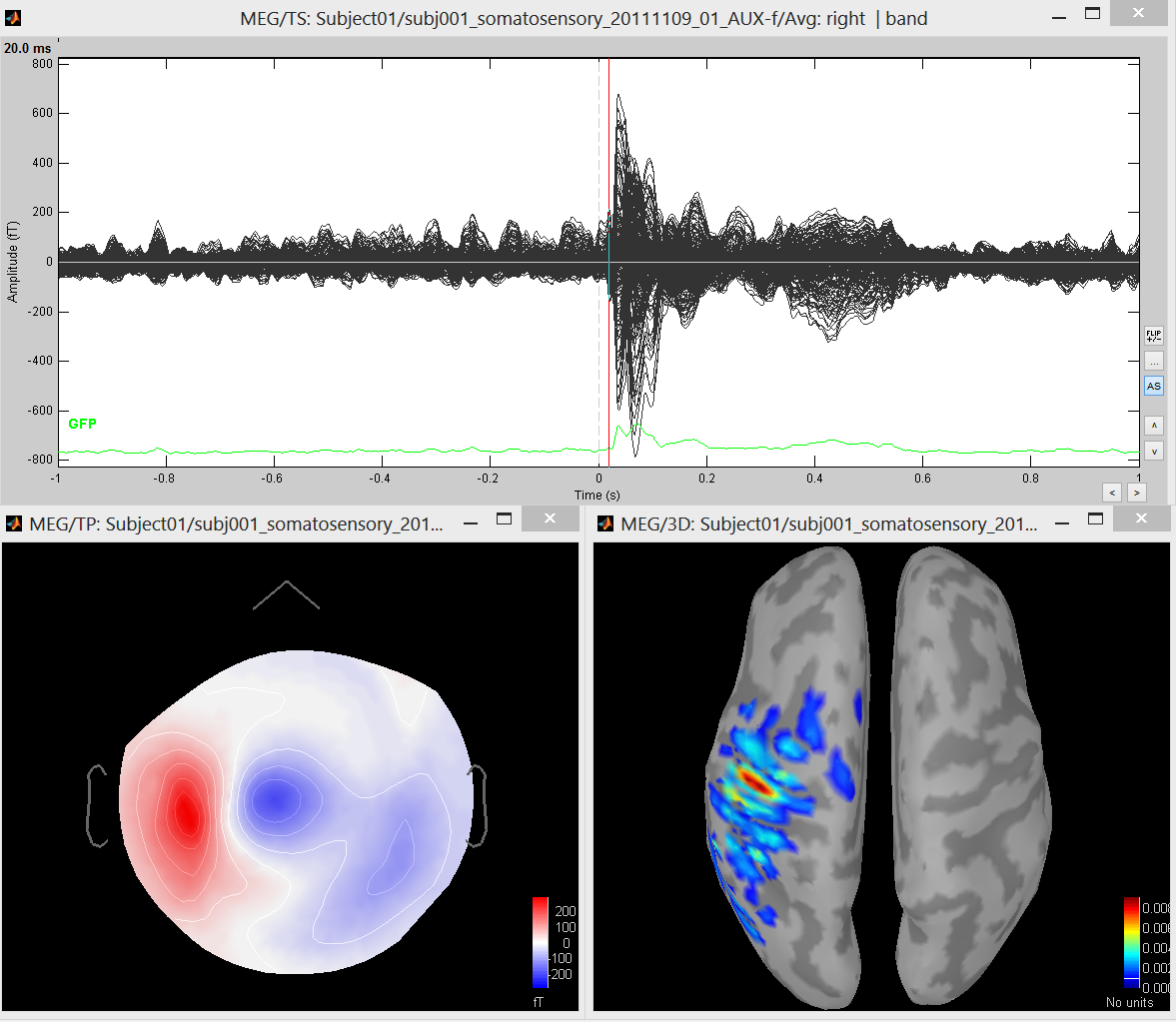
You will notice on the command window that a unique time-frequency box has been used (at scale j = 3 i.e. oscillations in the 37-75 Hz frequency band, peak of the wavelet located at 0.020 seconds). This oscillation is part of the short duration oscillatory pattern occurring at 20 msec.
Other suggestions:
run the wMEM with the same parameters as before but with scale = 4 ;
run the wMEM with the same parameters as before but with the scale = all. Then, you will combine all the boxes (3 boxes in all) that are above the time window you have selected:
with the previous choice of scales (all), run wMEM with the time window for 0.0 to 0.150 s (this time, the whole MNS response will localized using only 22 selected time-frequency boxes).
Parameters of wMEM
● Clustering: wavelet-adaptive
● MSP scores threshold: FDR method
rMEM
You have clicked on rMEM. The panel then displays all the parameters associated with this method. Parameters are defined in two sets:
The left column proposes basic mandatory parameters that will allow you to customize the localization of synchronous sources to your particular dataset.
The right column proposes more subtle parameters, for more advanced users. To access this set of parameters, you need to click on the ‘expert’ option. The ‘OK’ will be then available once all mandatory parameters have been specified. Please note that the default options regrouped under ‘model’, ‘wavelet’, and ‘ridges’ were carefully validated, we thus recommend not modifying them.
Principle: The signal is decomposed into continuous time-frequency plane using analytic Morse wavelets, the parameters of which appear in the right column, section ‘wavelet’. We then extract multivariate ridges from these planes, which are essentially the time-frequency location of the wavelet coefficients that are maximum along time. They exhibit specifically the synchronous content of the signal. Using these ridge lines, we then extract the complex wavelet coefficients that now define a multivariate “ridge signal”. Note that here ridge signals, just as any recording, appears in brainstorm with the following icon . The sources of these complex signals are then localized using MEM, and the results file appears under the corresponding ridge signal following the icon . As the ridges reflect synchronous signal components, the rMEM targets synchronous sources.
With the BEst_tutorial_median_nerve, we propose the following first experiment (similar to the cMEM, wMEM, previous experiment)
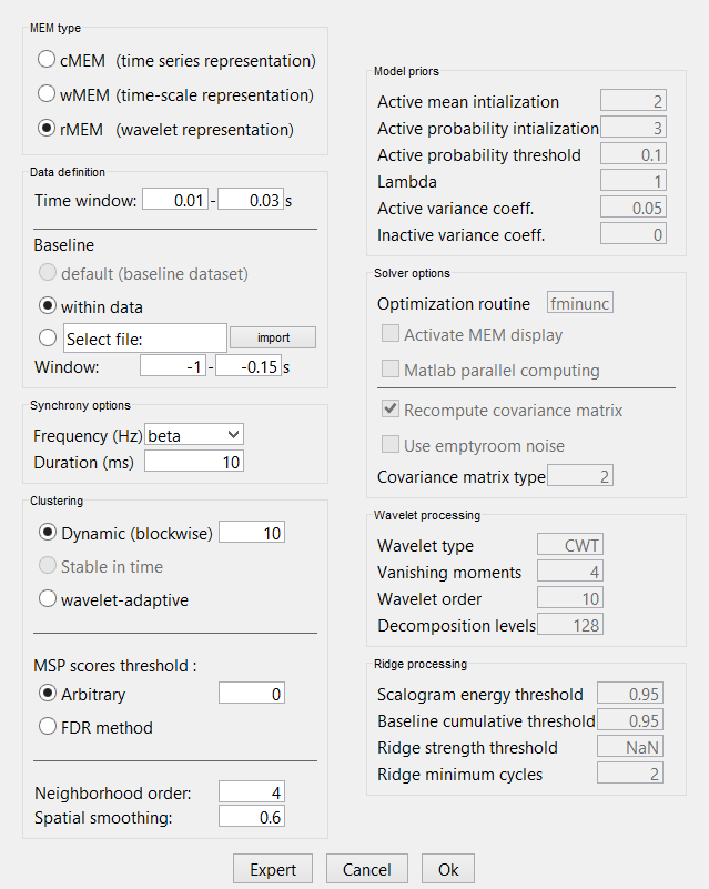
1. Selection of a specific time window may be useful to localize specific synchronous components of the recordings (default: localize synchrony in the whole data window). Suggested time window for this dataset: 0.010s to 0.030s.
2. Three choices are available for baseline definition.
Default: the panel looks for a dataset called 'baseline' within the same study as the data to be localized. When not found, this option is disabled. Within data: the baseline is a time window within the recordings. Import: the user can import baseline data from a file using brainstorm import tools In all cases, the user can define a time window for the baseline Suggested baseline for this dataset: within data, with interval -1 to -0.150 s
3. Selection of frequency band on interest. Suggested beta (13 to 29 Hz)
4. Selection of the duration criterion. Only synchrony lasting longer than threshold will be considered for source localization. Suggested 10 ms
5. MSP Scores Threshold: Arbitrary: 0.1
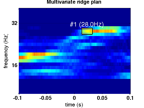
- This figure is the multivariate ridge plane computed with the parameters suggested. Each point shows the strength of the synchrony at a given time-frequency point. The ridge line extracted in the suggested time window is highlighted using a yellow box. This ridge line indexes the time-frequency coefficients that embody the synchronous oscillations in the beta-band during the time window of interest. In order to display this figure, you need to select the newly created time-frequency plane under the original data set and type in the command window:
be_vizr;
Optional syntax: be_vizr Flims [10 40]; xlim([-.1 .1])
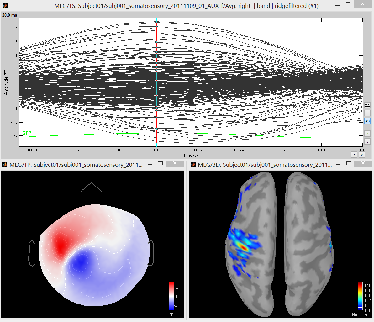
6. Hitting 'Ok' will launch the rMEM method. At the end, a new dataset, corresponding to the extracted ridge signal, and a results file appear in the database. Simply double-click them to visualize.
7. At the end of source localization, you may want to reload the brainstorm studies, this ensures that the new dataset and results file are displayed correctly in the brainstorm interface
Parameters of rMEM
● Clustering: dynamic or wavelet-adaptive
● MSP scores threshold: Arbitrary or FDR method
License
BEst is free software: you can redistribute it and/or modify it under the terms of the GNU General Public License as published by the Free Software Foundation, either version 3 of the License, or (at your option) any later version. BEst is distributed in the hope that it will be useful, but WITHOUT ANY WARRANTY; without even the implied warranty of MERCHANTABILITY or FITNESS FOR A PARTICULAR PURPOSE. See the GNU General Public License for more details. You should receive a copy of the GNU General Public License along with BEst. If not, get it here.
minFunc. Schmidt M. see license
References
The references to be acknowledged for each method are:
cMEM with stable clustering. MEG source localization of spatially extended generators of epileptic activity: comparing entropic and hierarchical bayesian approaches. Chowdhury RA, Lina JM, Kobayashi E, Grova C. PLoS One. 2013;8(2):e55969
wMEM. Wavelet-based localization of oscillatory sources from magnetoencephalography data. Lina J, Chowdhury R, Lemay E, Kobayashi E, Grova C. IEEE Trans Biomed Eng. 2012 Mar 6.
rMEM. Localization of synchronous cortical neural sources. Zerouali Y, Herry CL, Jemel B, Lina JM. IEEE Trans Biomed Eng. 2013 Mar;60(3):770-80.
Additional technical references:
MEM. Biomagnetic source detection by maximum entropy and graphical models. Amblard C, Lapalme E, Lina JM. IEEE Trans Biomed Eng. 2004 Mar;51(3):427-42.
MEM and Parcelization: Data-driven parceling and entropic inference in MEG. Lapalme E, Lina JM, Mattout J. Neuroimage. 2006 Mar;30(1):160-71.
MSP. Multivariate source prelocalization (MSP): use of functionally informed basis functions for better conditioning the MEG inverse problem. Mattout J, Pélégrini-Issac M, Garnero L, Benali H. Neuroimage. 2005 Jun;26(2):356-73.
Validation and applications:
Evaluation of EEG localization methods using realistic simulations of interictal spikes. Grova C, Daunizeau J, Lina JM, Bénar CG, Benali H, Gotman J. Neuroimage. 2006 Feb 1;29(3):734-53.
Concordance between distributed EEG source localization and simultaneous EEG-fMRI studies of epileptic spikes. Grova C, Daunizeau J, Kobayashi E, Bagshaw AP, Lina JM, Dubeau F, Gotman J. Neuroimage. 2008 Jan 15;39(2):755-74
Spatial correlation of hemodynamic changes related to interictal epileptic discharges with electric and magnetic source imaging. Heers M, Hedrich T, An D, Dubeau F, Gotman J, Grova C, Kobayashi E. Hum Brain Mapp. 2014 Feb 24.
Optimal eye-gaze fixation position for face-related neural responses. Zerouali Y, Lina JM, Jemel B. PLoS One. 2013 Jun 6;8(6):e60128.
Oscillatory activity in parietal and dorsolateral prefrontal cortex during retention in visual short-term memory: additive effects of spatial attention and memory load. Grimault S, Robitaille N, Grova C, Lina JM, Dubarry AS, Jolicoeur P. Hum Brain Mapp. 2009 Oct;30(10):3378-92.
MEM Parameters
Clustering
The major prior of the MEM is that cortical activity is compartmented into discrete parcels. The activity of a given source within a patch is thus linked to the activity of its neighbors. This step is thus important for the MEM approach and we propose some strategies to optimize it, depending on the type of activity we target for source localization. All these approaches are data-driven and consist mainly in two steps: sources scoring and labelling.
Source scoring: MSP
We first attribute a score to each source indicating its probability of explaining a segment of data. These scores are estimated using the multivariate source prelocalisation technique - MSP (Mattout et al. Neuroimage 2005). The MSP proceeds by computing a signal space projector using the SVD of the normalized data segment. The leadfields of each source are then normalized and projected on that space. The L2 norm of that projection thus gives a probability-like index between 0 and 1 weighting the contribution of each source to the data.
The MSP quantifies the probability for each source to explain some variability in a data segment. Implicitly, we expect MSP scores to discriminate active regions from inactive ones in relation to the analyzed data window. MSP aims at identifying good candidate dipolar sources contributing to the localization, with great sensitivity, but relatively low specificity. In this regard, the size of the data window on which MSP is applied is an important issue. If it is too short, the variability to be explained is low and all sources will have low scores. On the opposite, if it is too large, all sources will have high MSP scores. We thus propose three strategies to obtain appropriate MSP scores distributions:
- Stable in time
- Dynamic (blockwise)
- Wavelet-adaptative
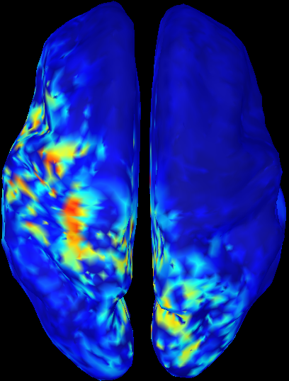
MSP scores of cMEM on MNS data (0.005-0.025s)
Source labelling: spatial clustering
The aim of this step is to group cortical sources into spatially homogenous cortical parcels based on their MSP scores. The clustering algorithm selects the sources with maximal MSP score, which are considered as seed points. The parcels are then constructed using a region growing algorithm starting from those seed points. It proceeds as follows:
- Select the source with maximal MSP score: it is the first seed point
- Select all the sources around the seed point to form a cluster. The size of the cluster is determined by the 'neighborhood order' value
- Amongst the other sources, we select the source with maximal MSP score, which will be the next seed point
- We repeat steps 2-3 until all the sources belong to a cluster
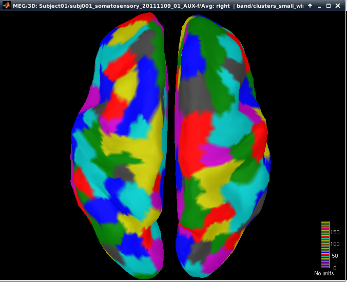
Clustering with neighborhood order of 4 (cMEM on MNS data)
MSP scores threshold
It is possible to apply a threshold on the MSP scores before applying the spatial clustering. All the sources that have MSP score below this threshold are then excluded and will not be part of any cluster and of the reconstructed sources. The threshold can be set arbitrarily from 0 to 1, 0 excluding none of the sources.
The MSP threshold can also be derived from the baseline using a FDR criterion. (Lina et al. IEEE TBME 2012)
Neighborhood order
The neighborhood order determines the size of the parcels in the spatial clustering. The neighborhood order relates to the number of maximal spatial connections along the geodesic cortical surface between an element of a cluster and the seed of this cluster. Therefore, the higher the neighborhood order, the larger the cluster and the lower the number of parcels. (Chowdhury et al. Plos One 2013, page 3)
Spatial smoothing
We can apply a spatial smoothing constraint (LORETA like) within each parcel during the MEM regularization. The parameter of smoothing can vary from 0 (no spatial smoothing) to 1 (high spatial diffusion inside the parcels). (Chowdhury et al. Plos One 2013, page 3 & 4, Harrison et al. Neuroimage 2007)
Expert parameters
Model prior
For the definition of the MEM prior model i.e., spatial clustering, the distribution of source intensities within each active parcel are modeled using a Gaussian distribution with a mean (mk) and a variance (Σk). The proposed prior model consists in using a hidden variable tuning the active state of each parcel. The probability of every parcel for being active has to be initialized as well (αk). The parameters of the active parcels can be initialized using different ways.
Active mean initialization (default choice, 2): Initialization of source intensity within each parcel.
- 1: mean of the source intensities computed by the weighted minimum norm scores of the sources within each parcel (mk = mean(Jmn)),
- 2: null initialization (mk = 0),
- 3: mean of the source intensities computed with a cluster-based version of the weighted minimum norm,
- 4: L-curve optimized minimum norm estimate.
Active probability initialization (default choice, 3): Initialization of the probability of the parcels being active (αk).
- 1: mean of MSP scores of the sources within each parcel,
- 2: max of MSP scores,
- 3: median of MSP scores,
- 4: all parcels initialized at 0.5,
- 5: all parcels initialized at 1.
Active probability threshold (default choice, 0): Parcels with sub-threshold initial probability are turned off. Parcels that are turned off cannot be part of the MEM solution.
Lambda (default choice, 1): Initial sensor’s weights vector.
- 0: all sensors initialized at 0,
- 1: random weights
Active variance coefficient (default choice, 0.05): model of variance of the active state. By default, variance is set to 5% of the mean of the square of the minimum norm estimate in each parcel. This proportion can be changed by setting active variance coefficient to desired value between 0 and 1.
Inactive variance coefficient (default choice, 0): model of variance of the inactive state.
Solver options
Optimization routine (default, fminunc): Optimization routine used for the MEM. Two toolboxes are available.
fminunc: Unconstrained optimization, part of the matlab optimization toolbox,
minFunc: Unconstrained optimization, copyright Mark Schmidt (selected when the optimization toolbox is not available).
Recompute covariance matrix: If this option is checked, a new covariance matrix will be recomputed instead of using the sensors covariance matrix already computed in brainstorm.
Use Empty room noise: This option is available when there is empty room noise available in the database. If you want this option to be available, the Brainstorm protocol must contain a dataset named “emptyroom”. The panel will look for “emptyroom” in the following order: 1) in the same study as the dataset to be localized, 2) in the subject node, 3) in the default subject node.
Covariance matrix type (default choice, 2): Only relevant if Recompute covariance matrix is checked.
- 0: identity matrix,
- 1: diagonal matrix, all sensors have same variance,
- 2: diagonal matrix,
- 3: full matrix
- 4: wavelet-based estimation of the noise. We compute the discrete wavelet transform of the data and estimate the noise from the finest scale, j=1. Note that the shrinkage is applied if selected. The matrix is diagonal.
SPECIFIC TO wMEM:
If there exists an emptyroom datasets and the option “Use emptyroom” is selected, the wMEM computes a scale-specific covariance matrix and a scale-dependent shrinkage (if selected). In this case, only options 4 and 5 are available and take a different meaning:
o 4: diagonal scale-specific covariance matrix – different values along the diagonal
o 5: (default – forced if neither 4 nor 5) diagonal scale-specific covariance matrix – unique value along the diagonal, which is the average of the diagonal terms
SPECIFIC TO rMEM:
If any of the options 1, 2 or 3 is selected, the noise covariance matrix is computed based on the ridge analysis of the baseline. First, we compute the continuous wavelet transform of the baseline. Then we extract the ridge b(t)=a, where a is the central frequency of the ridge signal to be localized. We read the wavelet coefficients along b(t), which is the baseline ridge signal, and compute the covariance matrix of this new signal. The meaning of options 1, 2 and 3 remains unchanged.
Wavelet Processing
Wavelet type
- CWT - Continuous Wavelet Transform (Morse) used for rMEM
- RDW - Discrete Wavelet transform (Real Daubechies) used for wMEM
Vanishing moments (default, 4): Number of vanishing moments of the wavelet. This parameter shapes the impulse response function of the wavelet. The larger this number, the more de-correlated are the coefficients, but the lower is the spectral resolution
Coefficient shrinkage (default, 1): Only relevant if Wavelet type is set to RDW. Indicates if the coefficients of the time-scale plane must be shrinked, used for data reduction.
Decomposition levels (default, 128): Only relevant if Wavelet type is set to CWT. Number of decomposition levels.
Ridge processing
Scalogram energy threshold (default, 0.95): Ridge maps are computed from the normalized scalogram by extracting local maxima of energy. This quantity limits the search for maxima to a percentage of total energy of the time-frequency plane. Recommended to leave it to default value.
Ridge strength threshold (default, NaN): Threshold on ridge strength, e.g. synchrony strength to avoid localizing poorly significant synchronous events. This quantity is normalized between 0 and 1. This threshold can be set to
- Arbitrary threshold between 0 and 1,
- Adaptive threshold (NaN), the threshold is learned from the baseline.
Baseline cumulative threshold (default, 0.95): Only relevant if Ridge strength threshold is set to NaN. All ridges from the baseline are extracted and the cumulative distribution of their strength is computed. The Ridge strength threshold will be interpolated at the Baseline cumulative threshold th percentile of that distribution.
Ridge minimum cycles (default, 2): Number of cycles within MSP. The size of the MSP window is set to Ridge minimum cycles times the number of samples covered by an oscillation at the frequency of the ridge to be localized. Only available for wavelet-adaptive clustering.

