Creation of figure from script

Hello,

I recently tried to automatized some of the plot made in Brainstorm. I am able to make the figure i want using the following script :

for Hb = {'HbO', 'HbR','HbT'}
    [hFig, iDS, iFig] = script_view_sources(sMNE(contains({sMNE.Comment},Hb{1})).FileName, 'cortex');
    figure_3d('SetStandardView',hFig, 'top');
    panel_surface('SelectHemispheres', 'right');
    panel_time('SetCurrentTime', time_of_snapshot);
    bst_colormaps('SetColormapName',      'nirs', "cmap_mandrill");
    bst_figures('SetBackgroundColor',hFig, [1 1 1]) 
    panel_scout('PlotScouts',1, hFig)
    hColorbar = findobj(hFig, 'Tag', 'Colorbar');
    hColorbar.Position=[400 30 15 90];
    bst_report('Snapshot', hFig,           sMNE(contains({sMNE.Comment},Hb{1})).FileName,sprintf('MNE - %s',Hb{1}),hFig.Position)
end

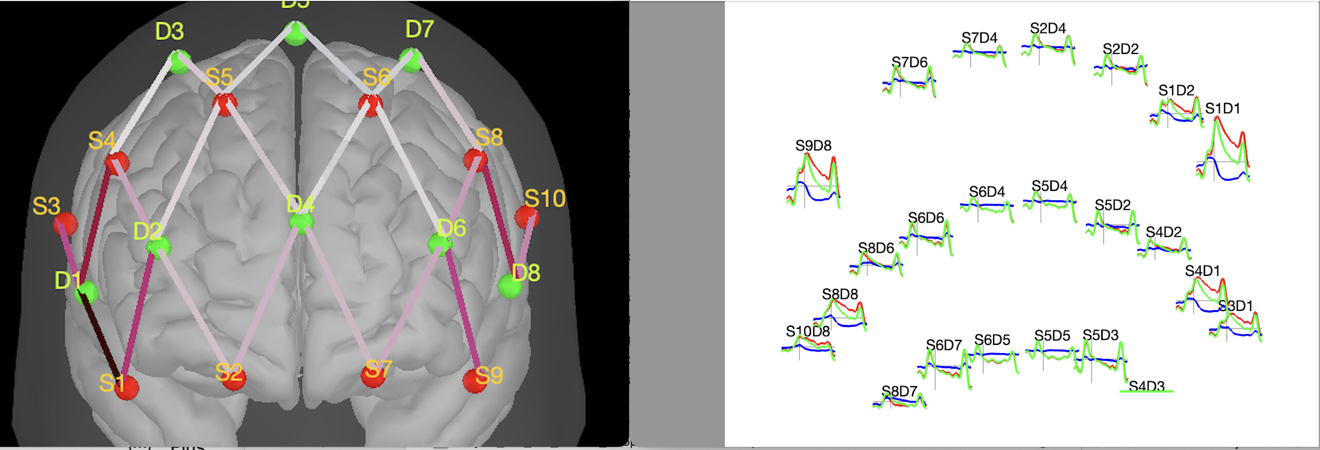
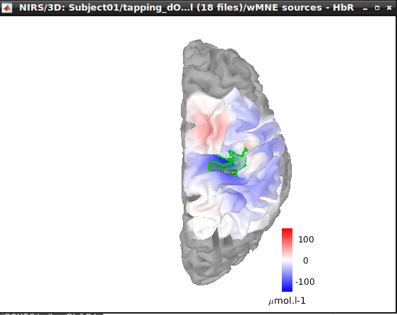
where sMNE contains some source maps. Te maps are displayed are expected but if i look in the report. The scout that are displayed in the figure 1 disappear in the report (figure 2)

snapshot_figure

snapshot_report

Questions:

  1. Is there any solution to make sure that the scout is also displayed in the report?

  2. Also, i was wondering how can i view the scout time series from script ?
    i tried ''' hFig = view_scouts({sMNE(contains({sMNE.Comment},'HbO')).FileName}, 'hand') ''' but without success.

Solutions:

  1. No solution yet. but interestingly. Saving the image using : out_figure_image( hFig, fullfile(reports_dir, sprintf('%s-%s.tiff',map_leg, Hb{1}))) works

  2. panel_scout('SetScoutsOptions',1, 1, 0, 'all', 1, 1, 0, 0); . hFig = view_scouts({sMNE(contains({sMNE.Comment},{'HbO','HbR'})).FileName} , 1)

Regards,
Edouard

2 Likes

thanks for the formatting edit @Raymundo.Cassani. I re-edited to clarify that issue 1 is not solved yet :slight_smile:

Hi @edelaire ,

A way to show the scouts in the report figure is to bypass bst_report('Snapshot')

  1. Create your own image from Figure already showing the scouts:
    img = out_figure_image(hFig);

  2. Add this image to the report:
    bst_report('Add', 'image', sFile.Comment, sFile.Filename, img);

BTW, in the bst_report('Snapshot') the scouts are hidden here: brainstorm3/toolbox/process/bst_report.m at b2ce2e3c3b101fc74f774557d2bcf9fd7e3cceb2 · brainstorm-tools/brainstorm3 · GitHub

1 Like

Thanks. it is working. However, i noticed a weird behavior (maybe not linked to Brainstorm).
Following code is able to add the figure in the report; but the image doesnt seems to be created on the disk..

[hFig, iDS, iFig] = view_timeseries(sAverageDOD.FileName, 'NIRS',[], 'NewFigure');
img = out_figure_image( hFig, fullfile(reports_dir,  sprintf('%s-%s.tiff','avg_timeseries_plot', 'dOD')),'');
bst_report('Add', 'image', sprintf('%s-%s.tiff','avg_timeseries_plot', 'dOD'), sAverageDOD.FileName, img);    
close(hFig)
% OUT_FIGURE_IMAGE: Save window contents as a bitmap image.
%
% USAGE: img = out_figure_image(hFig)           : Extract figure image and return it
%              out_figure_image(hFig, imgFile)  : Extract figure image and save it to imgFile

If there is an output variable: out_figure_image returns the captured image as a RGB array and ignores the parameter imgFile.
The images are saved as RGB arrays in the reports, and saved in the HTML file in the same way when exporting them.

1 Like

Thanks you. It's working. I have another question regarding the creation of figures from scripts (hope it's ok to regroup all of them here).

Questions:

  1. When creating a 2D layout. How can I display the channel label from this script?
[hFig, iDS, iFig] = view_topography(data.FileName, 'NIRS', '2DLayout');
panel_montage('SetCurrentMontage',hFig, sprintf('%s[tmp]', 'NIRS overlay'))
bst_figures('SetBackgroundColor',hFig, [1 1 1])
  1. The figure is quite hard to read with a white background; is there any way to avoid the black background while still making the graph nice to read?

Black Background:
subject_HW_105_task_Dual_pre_2D_layout.tiff (117.4 KB)

White Background:

subject_HW_105_task_Dual_pre_2D_layout.tiff (125.0 KB)

  1. The file I am trying to display is an average with standard deviation. Would it be possible to have also the std displayed on the graph for each channel?

  2. Is it possible to change the orientation of the graph. (see bellow). In general it seems very hard to make the correspondance between the montage and the 2D layout as left is right and top is front. (I never realised that until now)

Solutions:

  1. The two followings code works (i prefer the second one :p)
global GlobalData;
set(GlobalData.DataSet(iDS).Figure(iFig).Handles.hSensorLabels, 'Visible', 1);                

or
set(findobj(gcf,'Tag','SensorsLabels'),'Visible', 'on');

  1. The following code help; but don't know if it possible to do better :slight_smile:
set(findobj(gcf,'Tag','SensorsLabels'),'Color',[0,0,0]);
set(findobj(gcf,'Tag','SensorsLabels'),'FontSize',FontSize); % 14 instead of 9
set(findobj(gcf, 'Tag' , 'Lines2DLayout'),'LineWidth', 2);

subject_HW_105_task_Dual_pre_2D_layout.tiff (193.9 KB)

  1. WIP

  2. Current WIP:
    The 2D layout make sense if we look at the montage from at top view; but still for a montage on the frontal lobe; that's a bit weird and it would be great to be able to change it :slight_smile:
    axis ij correct the left-right orientation

I tried to play with set ( gca, 'xdir' / 'ydir', /'zdir', 'normal' / 'reverse') but doesn't work. Still x is always up:

What is really weird is that with this toy example (see bellow), it is very easy to change axis direction in any way we want; but with brainstorm figure it seems that x- and y- axis are linked so X is always pointing up.

figure;
hold on;
quiver3(0,0,0,1,0,0); text(0.8,0,0,'x');
quiver3(0,0,0,0,1,0); text(0,0.8,0,'y');
quiver3(0,0,0,0,0,1); text(0,0,0.8,'z');

set(gca, 'XDir','normal') % or 'reverse'
set(gca, 'YDir','normal')
set(gca, 'ZDir','normal')

Following code correctly place the plots but then all the curve are also inverted (eg an increase is plot as a decrease)... An easy solution would be to multiply all data by -1 before the plot :slight_smile:

tmp = findobj(gcf, 'Tag' ,'Axes3D')
set(tmp, 'CameraUpVector', [-1 0 0])

ok; it's 1am now; I think I spent way too much time on this ahah but following code works(almost) (it's ugly - however) :

                panel_montage('SetCurrentMontage',hFig, sprintf('%s[tmp]', 'NIRS overlay'))
                bst_figures('SetBackgroundColor',hFig, [1 1 1]) %- white background is ugly
                set(findobj(gcf,'Tag','SensorsLabels'),'Visible', 'on');
                set(findobj(gcf,'Tag','SensorsLabels'),'Color',[0,0,0]);
                set(findobj(gcf,'Tag','SensorsLabels'),'FontSize',FontSize);
                set(findobj(gcf, 'Tag' , 'Lines2DLayout'),'LineWidth', 2);
                set(findobj(gcf, 'Tag' ,'Axes3D'),'CameraUpVector', [-1 0 0])

                tmp = findobj(gcf, 'Tag' ,'Lines2DLayout');
                tmp2 = findobj(gcf, 'Tag','2DLayoutZeroLines');
                for i_curve = 1:length(tmp)
                    set(tmp(i_curve),'XData', 2*tmp2(i_curve).XData(1) -1*(tmp(i_curve).XData))
                    set(tmp(i_curve),'YData', tmp(i_curve).YData(end:-1:1))
                end
                panel_time('SetCurrentTime', 25);

Note: we have to specify 25 instead of 0 because the X axis is reversed now...

actually, here is final code (for some reason, some change are not applied the first time; so need to execute code twice; also need to adjust the coordinate of the label)....

            % Figure 3. 2D Layout
            for wtf = 1:2 % for some reason the code needs to be repeated 2 times; otherwise background doesnt work
            [hFig, iDS, iFig] = view_topography(data.FileName, 'NIRS', '2DLayout');
                pause(1)
                panel_montage('SetCurrentMontage',hFig, sprintf('%s[tmp]', 'NIRS overlay'))
                set(findobj(gcf,'Tag','SensorsLabels'),'Visible', 'on');
                set(findobj(gcf,'Tag','SensorsLabels'),'Color',[0,0,0]);
                set(findobj(gcf,'Tag','SensorsLabels'),'FontSize',FontSize);
                bst_figures('SetBackgroundColor',hFig, [1 1 1]) %- white background is ugly
                set(findobj(gcf, 'Tag' , 'Lines2DLayout'),'LineWidth', 2);
                set(findobj(gcf, 'Tag' ,'Axes3D'),'CameraUpVector', [-1 0 0])

                tmp = findobj(gcf, 'Tag' ,'Lines2DLayout');
                tmp2 = findobj(gcf, 'Tag','2DLayoutZeroLines');
                tmp3 = findobj(gcf,'Tag','SensorsLabels');

                for i_curve = 1:length(tmp)
                    set(tmp(i_curve),'XData', 2*tmp2(i_curve).XData(1) -1*(tmp(i_curve).XData))
                    set(tmp(i_curve),'YData', tmp(i_curve).YData(end:-1:1))
                    
                    if wtf == 2
                        label_newPos = tmp3(i_curve).Position;
                        label_newPos(1) = 2*tmp2(i_curve).XData(1) - 1.01*(tmp3(i_curve).Position(1));
                        set(tmp3(i_curve),'Position', label_newPos);
                    end
                end
                panel_time('SetCurrentTime', 25);
            end
            out_figure_image( hFig, fullfile(reports_dir,  fname(subject_name,task,cond,'2D_layout')),'');
            close(hFig)

and final figure :face_with_spiral_eyes:
subject_HW_105_task_Dual_pre_2D_layout.tiff (193.7 KB)

Edouard

Edit: fix formating
An additional question (more important)

  • When displaying multiple 2D layouts, how can I make sure that the scale is the same between all 2D layouts? Right now it seems that the scale is different so it's very hard to compare the amplitude of different files

I tried to look at GlobalData.DataSet(iDS).Figure(iFig).Handles.DisplayFactor to then be able to use figure_topo('UpdateTimeSeriesFactor',hFig, factor) but its always 1... so very weird...

solution:
I solved it by computing the ratio between the max of the two files; then scaled the second file using that ratio with figure_topo('UpdateTimeSeriesFactor',hFig, factor)

When viewing the topography, how can we make sure that the color bar is the same accross figure? i tried a lot of thing, none work yet...

[hFig, iDS, iFig] = view_topography(data.FileName, 'NIRS', '3DOptodes',[],0,'NewFigure');
panel_montage('SetCurrentMontage',hFig, sprintf('%s[tmp]', Hb{1}))
panel_time('SetCurrentTime', time_of_snapshot);
bst_colormaps('SetColormapName',      'nirs', colormap_name);
bst_colormaps('SetColormapRealMin','source', 0)
bst_colormaps('SetMaxCustom','source', '\mumol.l-1', -1*200*1e-6,200*1e-6)
caxis(200 * [-1 1]*1e-6);

subject_HW_211_task_Dual_pre_3Doptodes-HbR.tiff (341.8 KB)

subject_HW_211_task_Single_pre_3Doptodes-HbR.tiff (343.2 KB)

the scale is just choosen randomly,,,

I thought the issue was because of the unit since the file is in micromol so has a scale of 10e-6. So i tried :

sData = in_bst_data(data.FileName);
sChannels = in_bst_channel(data.ChannelFile);

F = sData.F .* 1e6;

[hFig, iDS, iFig] = view_topography(data.FileName, 'NIRS', '3DOptodes',F,0,'NewFigure');

but then the data are not even plotted anymore and color doesn't change with montage or time

Even

[hFig, iDS, iFig] = view_topography(data.FileName, 'NIRS', '3DOptodes',sData.F,0,'NewFigure');

doesnt work when it should vie the exact same plot as [hFig, iDS, iFig] = view_topography(data.FileName, 'NIRS', '3DOptodes',,0,'NewFigure');

ok; i am stupid... the solution was

bst_colormaps('SetColormapRealMin','nirs', 0)
bst_colormaps('SetMaxCustom','nirs', '\mumol.l-1', -1*color_scale(Hb{1})*1e-6, color_scale(Hb{1})*1e-6)

(NIRS instead of source)

  1. The file I am trying to display is an average with standard deviation. Would it be possible to have also the std displayed on the graph for each channel?

Not at the moment. This requires major editing of figure_topo.m (functions GetFigureData and CreateTopo2dLayout at least).

In general it seems very hard to make the correspondance between the montage and the 2D layout as left is right and top is front.

Only if you configure your 3D figure with a front view. Use a top view and they are aligned.

What is really weird is that with this toy example (see bellow), it is very easy to change axis direction in any way we want; but with brainstorm figure it seems that x- and y- axis are linked so X is always pointing up.

You'd need to edit a lot of code in figure_topo.m.
I'm sorry, I don't have time to help you with this at the moment.

When displaying multiple 2D layouts, how can I make sure that the scale is the same between all 2D layouts? Right now it seems that the scale is different so it's very hard to compare the amplitude of different files

The values in 2DLayout are always normalized to the max of the data, therefore there is no solution to obtain the same graph for different files.
To compare the values from two files with this display mode: overlay the two files (select them simultaneously in the tree, or pass the two files as cell arrays to the display function).
Or use a different display mode (for time time series, the most appropriate is the time series figure).

When viewing the topography, how can we make sure that the color bar is the same accross figure?

Is this solved? I'm not sure I followed correctly what's below