Dear Experts,
I am a junior user of Brainstorm (BTW, congratulations for the tool).
I am inferring the functional connectivity in sources space with the Phase Transfer Entropy (PTE) NxN method using EEG data recorded during sleep.
The source activities, due to the computational complexity of the problem, is averaged before the PTE calculation in 148 scouts with Destrieux parcellation (scoutfunc=mean; scouttime=before). Since I don't have the MRI of the subjects I'm employing an MRI template. For this reason I'm using sources on the cortical surface with unconstrained orientation.
I tried 2 options, normalized PTE and non-normalized PTE but I'm having some trouble interpreting the results I get from the normalized PTE.
In the Figure attached I plotted an histogram of the obtained non-normalized (top-left) and normalized (top-right) PTE values of 1 control and 1 patient.
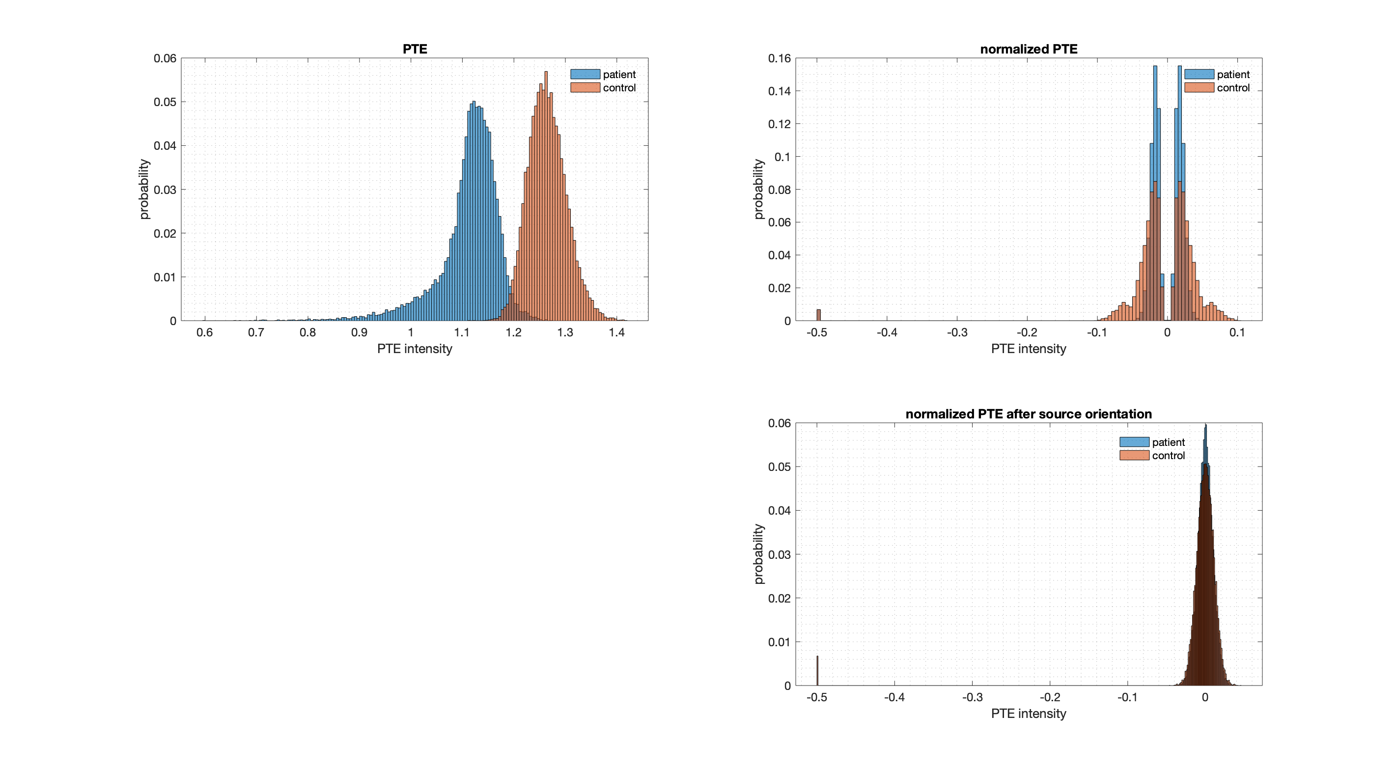
Since the graph on the right seemed strange to me I tried to invert the order in which the 2 operations of matrix normalization and source orientation are performed.
So instead of normalizing the PTE matrix (1483 x 1483) and then orienting the sources (absmax function) to get a normalized PTE matrix (148 x 148) I perform first the orientation (snippet 1) and only after the normalization (snippet 2).
Snippet 1 (bst_connectivity.m, line #620)
% Dimension #1
if isUnconstrA
[R, sInputA.GridAtlas, sInputA.RowNames] = bst_source_orient(, sInputA.nComponents, sInputA.GridAtlas, R, UnconstrFunc, sInputA.DataType, sInputA.RowNames);
end
% Dimension #2
if isUnconstrB
R = exchanges(R, [2 1 3 4]);
[R, sInputB.GridAtlas, sInputB.RowNames] = bst_source_orient(, sInputB.nComponents, sInputB.GridAtlas, R, UnconstrFunc, sInputB.DataType, sInputB.RowNames);
R = permutations(R, [2 1 3 4]);
end
Snippet 2 (PhaseTE_MF.m, line #142)
%% Compute dPTE
tmp = triu(PTE) + tril(PTE)';
dPTE = [triu(PTE./tmp,1) + tril(PTE./tmp',-1)];
The result by reversing the operations is shown in Figure (bottom-right)
which seems more interpretable to me.
What do you think? In the case of sources with unconstrained orientation, shouldn't one first orient and only then normalize?
Thank you very much for your support.
Kind regards
Max