How is the orthogonalization symmetric in the "bst_henv.m" function?

Hello,

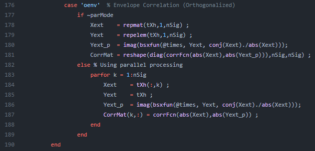
I was wondering how the orthogonalization is coded to be symmetric into the function "bst_henv.m". I find the following code in the .m file:

image

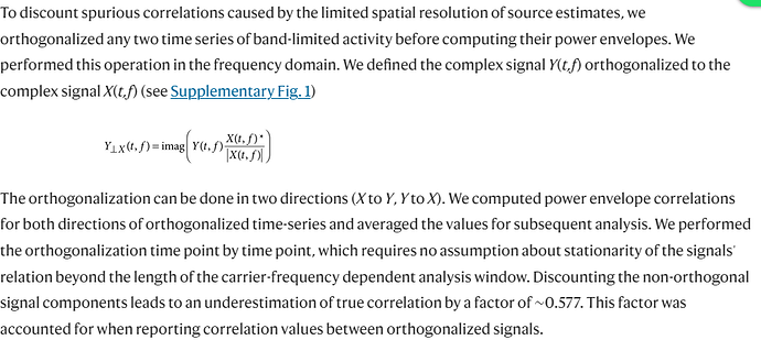
I recognize the orthogonalization method as the one in the article of Hipp et al. (2012):

But I can't really see the two orthogonalizations and the averaging afterwards. This is probably my lack of coding knowledge, but I am trying to learn it so any explanation would be helpful.

Thanks in advance!

This is a question for the author of the function: @hossein27en

Hi @gvh,

The two orthogonalizations happen in

Xext    = repmat(tXh,1,nSig) ;
Yext    = repelem(tXh,1,nSig) ;    
Yext_p  = imag(bsxfun(@times, Yext, conj(Xext)./abs(Xext)));

This operation is performed for each band, we can let aside the frequency dimension for now. Consider two (column vector) signals u and v with their corresponding analytic signals [ũ, ], and the variable tXh containing those signals, this is to say: tXh = [ũ, ]

Then, Xext is equal to [ũ, , ũ, ] , and Yext is equal to [ũ, ũ, , ] .
The operation is performed for each column vector, thus: Yext_p = [ũ⟂ũ, ũ⟂ṽ, ṽ⟂ũ, ṽ⟂ṽ]. Lastly, the correlation is computed and reshaped in

CorrMat = reshape(diag(corrFcn(abs(Xext),abs(Yext_p))),nSig,nSig) ;

In this case, CorrMat is a [2×2] matrix with:
[corr(|ũ|, |ũ⟂ũ|), corr(|ṽ|, |ũ⟂ṽ|) ; corr(|ũ|, |ṽ⟂u|), corr(|ṽ|, |ṽ⟂ṽ|)]


The average happens later in the line:

A(:,:,t,f) = (abs(CorrMat) + abs(CorrMat'))/2 ;

Best,
Raymundo

1 Like

I see, thank you very much for the clarification!

@Raymundo.Cassani

I have an additional question, but no pressure if you do not want to answer it. The averaging uses absolute values (indicated in the comment above it with the assumption that all measures are "non-negative"). How is it still possible to obtain negative AEC values?

Many thanks in advance!

The amplitude envelopes, |ũ| and |ṽ|, are not negative. However their correlation can take negative values.

Dear Raymundo.Cassani and Francois,

Recently, I conducted simulations on two signal segments and executed the code you provided:

t = 0:0.01:2*pi;
u = sin(t)';
v = cos(t)';
u_analytic = hilbert(u);
v_analytic = hilbert(v);
tXh = [u_analytic,v_analytic];
Xext    = repmat(tXh,1,2) ;
Yext    = repelem(tXh,1,2) ;    
Yext_p  = imag(bsxfun(@times, Yext, conj(Xext)./abs(Xext)));
CorrMat = reshape(diag(corr(abs(Xext),abs(Yext_p))),2,2) ;
A(: , :) = (abs(CorrMat) + abs(CorrMat'))/2 ;

The results I obtained are as follows:

0.067989	0.092222
0.092222	0.034612

However, according to your explanation, CorrMat is a [2×2] matrix with the elements:

[corr(|ũ|, |ũ⟂ũ|), corr(|ṽ|, |ũ⟂ṽ|) ; corr(|ũ|, |ṽ⟂u|), corr(|ṽ|, |ṽ⟂ṽ|)]

The diagonal elements of the correlation matrix should have a value of 1. However, it is evident that I did not obtain this result in my simulation.

Similarly, I also used the "HOrthCorr" function from "bst_henv.m" to calculate the orthogonalized envelope correlation.

t = 0:0.01:2*pi;
Xh = hilbert(cos(t))';
ConVec = HOrthCorr(Xh, Xh);

When both signals are perfectly identical, I obtained a correlation value of 0.067989.

As per my understanding, when the two signals are identical, the correlation should ideally be 1. However, the result I obtained seems to deviate significantly from this expectation. I would be extremely grateful if you could shed some light on this observation and help me comprehend the reasons behind this unexpected outcome. I want to ensure that my calculations are accurate and that I am correctly utilizing the "bst_henv.m" function.
If there are any specific considerations or steps that I might be missing in the process, please guide me through them to rectify the issue.
Thank you for your invaluable assistance, and I look forward to your insights.

Best regards,
Yanxi
Hi Yanxi,

This is not the case as the diagonal of the correlation matrix is not the correlation of a signal (|ũ|) with itself, but with itself orthogonalized by itself ( |ũ⟂ũ|). Thus the results is not 1.

This is the same code with comments, I hope it helps:

t = 0:0.01:2*pi;
u = sin(t)';                    
v = cos(t)';
u_analytic = hilbert(u);
v_analytic = hilbert(v);
% u, v, u_analytic and v_analytic as column vectors: size [nSamples, 1] each

tXh = [u_analytic,v_analytic];
Xext    = repmat(tXh,1,2) ;
% Xext = [u_analytic, v_analytic, u_analytic, v_analytic];

Yext    = repelem(tXh,1,2) ;    
% Yext = [u_analytic, u_analytic, v_analytic, v_analytic];
% Same signals as in Xext but in different order

Yext_p  = imag(bsxfun(@times, Yext, conj(Xext)./abs(Xext)));
% Yext_p is each column of Yext orthogonalized by its respective column in Xext
%  Yext_p = [u_analytic⟂u_analytic, u_analytic⟂v_analytic, v_analytic⟂u_analytic, v_analytic⟂v_analytic];

CorrMat = reshape(diag(corr(abs(Xext),abs(Yext_p))),2,2) ;
% corr(abs(Xext),abs(Yext_p)) give as 4x4 matrix, but we are only interested in the correlation of Xext(i,:) with Y(i,:) for i = 1:4, thus we keep only the diagonal, and reshape it as [2,2]

A(: , :) = (abs(CorrMat) + abs(CorrMat'))/2 ;
% Average corr matrix to make symmetrical

Dear Raymundo.Cassani ,

Thanks for your patient response. It has been really helpful to me.
Regarding the matter, I have another question. Is it possible to set the diagonal of the relevance matrix to zero? I noticed in version 230724 of Brainstorm, there are lines 194-195 in the 'bst_henv.m' function where the diagonal of the correlation matrix is set to zero, but these lines seem to be commented out. I'm wondering if a similar approach can be applied for orthogonalizing the envelope correlation.
I eagerly await your response and appreciate your continued support.
Thank you once again for your patience and guidance.

Best regards,
Yanxi