Greetings everybody,
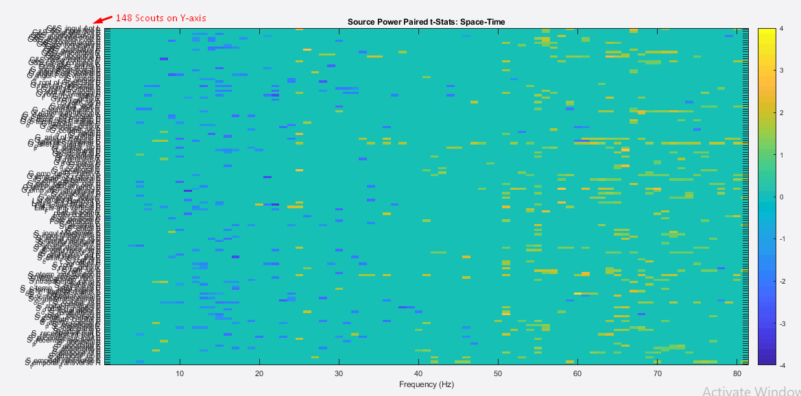
We have computed the subject wise single trial PSDs on source level for each of the two conditions (space and time) of study. Then we ran the paired t-test on average source PSDs of 17 subjects for the group analysis across two conditions. To visualize the results and significant values we exported the paired t-Test results to Matlab which resulted in the following attached image 1. Here we observed several significant scouts at different frequencies. It is possible to see the individual scouts on anatomical maps.
But our question is, how can we inspect and visualize the significant clusters of scouts at different frequencies on anatomical maps by projecting the sources to default anatomy, in the group analysis?
Any help would be really appreciated. Thank you!
Best regards,
Abrar
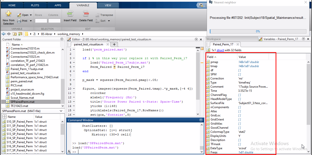
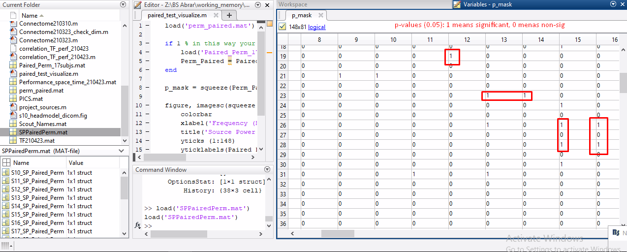
For reference, MATLAB script and paired t-test images are attached, and the pipeline of Source Estimation and Stats in source space includes the following steps;
- Data and noise covariance.
- Compute head model (OpenMEEG BEM).
- Compute sources (Single trials, LCMV Beamformer, PNAI: MEG GRAD, Full, constrained, Destrieux atlas-148 scouts).
- Compute single trial source PSDs across two conditions.
- Compute subject average source PSD across two conditions.
- Permute paired t-stats on subjects average source PSDs (with average over time).
- Visualize results of t-maps and p-maps in Matlab by exporting the resultant file of t-test.