Scout function in PLV calculation

Junichi_Uemura · December 10, 2015, 11:25pm

Hi all,

I’m planning to calculate the PLV with ‘Mean’ scout function. My question is how to calculate the PLV with ‘Mean’ scout function.
Is this based on the PLV with ‘All’ scout function?

Best,
Jun

Francois · December 11, 2015, 12:53pm

Hi Jun,

It’s like all the connectivity and time-frequency functions: it depends what you select for the option “When to apply the scout function”.
If you choose “before”: It computes the mean of the vertices for scouts S1 and S2, then compute the connectivity metric S1xS2.
If you choose “after”: It computes the connectivity metric for all the pairs of vertices in S1 and S2, you get a matrix [N1 x N2], then it applies the scout function (“mean”) to all the values in this matrix, to return only one value for PLV(S1,S2).

Cheers,
Francois

Junichi_Uemura · December 12, 2015, 3:36am

Hi Francois,

I chose “after” option.
I exported a matrix [N1 × N2] computed by applying the scout function “All”. Then, I calculated the mean of all values in this matrix on Excel. The mean value which I got on Excel is different from the one computed by applying the scout function “mean”. Is it correct? I suspect that the scout function “mean” is not working correctly. I use the newest version.

Best,
Jun

Francois · December 12, 2015, 3:57am

Hi Jun,

Make sure you process the different frequency bands separately.
The code to process the scout values for the connectivity functions is quite convoluted, so it is possible that there are errors in it.
You place two breakpoints to follow what is happening in the code:

bst_connectivity, line 658
process_average_rows, line 339

Let me know if you find anything suspicious.

Cheers,
Francois

Junichi_Uemura · December 12, 2015, 4:31am

Hi Francois,

Yes, I processed the different frequency bands separately.
Though I can not do it now, I will check the code.

Best,
Jun

Junichi_Uemura · December 17, 2015, 12:01am

Hi Francois,

I placed two breakpoints to follow what was happening in the code:

bst_connectivity, line 658
process_average_rows, line 339

As I’m not familiar with Matlab, I can not find any errors. But if there are errors in it, I’m suspicious of

process_average_rows, line 317. 323. 336. 337. 342

I was wandering if you could check these lines for me.
Thank you in advance.

Best,
Jun

Francois · December 22, 2015, 2:26am

Hi Jun,

I tested this and could not find any difference between the two approaches: using the options “Mean/After” or “All+averaging manually”.
Please note that averaging these values manually requires a lot of scripting, as show in the examples below.

Using scout options “Mean/After”:

% Process: Phase locking value NxN
sFilesPlvMean = bst_process('CallProcess', 'process_plv1n', sFiles, [], ...
    'timewindow', [-0.1, 0.5], ...
    'scouts', {'User scouts', {'A1', 'IFG'}}, ...
    'scoutfunc', 1, ...  % Mean
    'scouttime', 2, ...  % After
    'freqbands', {'delta', '2, 4', 'mean'; 'theta', '5, 7', 'mean'; 'alpha', '8, 12', 'mean'; 'beta', '15, 29', 'mean'; 'gamma1', '30, 59', 'mean'; 'gamma2', '60, 90', 'mean'}, ...
    'mirror', 1, ...
    'keeptime', 0, ...
    'outputmode', 3);  % Save average connectivity matrix (one file)

Using scout option “All”:

% Process: Phase locking value NxN
sFilesPlv = bst_process('CallProcess', 'process_plv1n', sFiles, [], ...
    'timewindow', [-0.1, 0.5], ...
    'scouts', {'User scouts', {'A1', 'IFG'}}, ...
    'scoutfunc', 5, ...  % All
    'scouttime', 2, ...  % After
    'freqbands', {'delta', '2, 4', 'mean'; 'theta', '5, 7', 'mean'; 'alpha', '8, 12', 'mean'; 'beta', '15, 29', 'mean'; 'gamma1', '30, 59', 'mean'; 'gamma2', '60, 90', 'mean'}, ...
    'mirror', 1, ...
    'keeptime', 0, ...
    'outputmode', 3);  % Save average connectivity matrix (one file)

% Load file
sMat = in_bst_timefreq(sFilesPlv(1).FileName);
N = length(sMat.RowNames);
Nfreq = size(sMat.TF,3);
iVertS1 = 1:20;
iVertS2 = 21:40;
% Expand connectivity matrix
sMat.TF = process_compress_sym('Expand', sMat.TF, N);
sMat.TF = reshape(sMat.TF, N, N, []);
% Average scouts
TFtmp = zeros(2,2,Nfreq);
for iFreq = 1:Nfreq
    TFtmp(1,1,iFreq) = mean(reshape(sMat.TF(iVertS1,iVertS1,iFreq),[],1));
    TFtmp(1,2,iFreq) = mean(reshape(sMat.TF(iVertS1,iVertS2,iFreq),[],1));
    TFtmp(2,1,iFreq) = mean(reshape(sMat.TF(iVertS2,iVertS1,iFreq),[],1));
    TFtmp(2,2,iFreq) = mean(reshape(sMat.TF(iVertS2,iVertS2,iFreq),[],1));
end
% Compress connectivity matrix
TFtmp = reshape(TFtmp, 2*2, 1, Nfreq);
TFtmp = process_compress_sym('Compress', TFtmp);
% Create new structure
sMat.TF = TFtmp;
sMat.RefRowNames = {'S1','S2'};
sMat.RowNames = {'S1','S2'};
sMat.ScoutFunc = 'mean';
sMat.Comment = [sMat.Comment, ' | AVG'];
% Add to database
db_add(sFilesPlv(1).iStudy, sMat);

Cheers,
Francois

Junichi_Uemura · December 24, 2015, 11:26pm

Hi Francois,

Thank you for your reply.
I might have a mistake with this process. Can I confirm it?

I will attach some pictures.

PLV_all_vertex(15): calculated PLV 'ALL'
PLV_mean_vertex(15): calculated PLV 'mean_after'
excel data: exported 'ALL' data on Excel

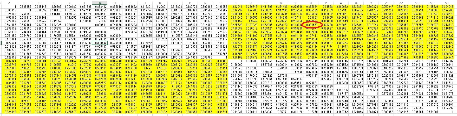
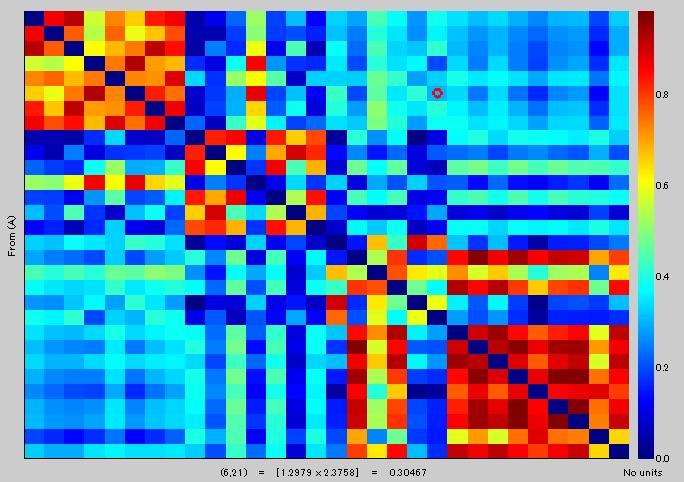
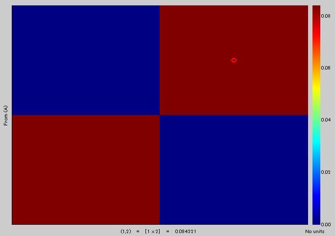
You can see that two values are the same [(6,21)=0.3046] in1), and red circle [(6,U)=0.3046] in 3).
Number of vertexes is 15.
Yellow area in 3) corresponds to red area in 2). Is it right?

Mean value of yellow area in 3) is 0.29399, but the value of red area in 2) is 0.084221. Is it correct?

I would be happy if you could give me some advices.

Thank you

Best,
Jun

Francois · January 3, 2016, 1:46am

Hi Jun,

I’m sorry, I cannot check how you manipulate your data in Excel.
If you think there is something wrong with this process, could you please illustrate it with a piece of Matlab code that I could run on my end?

Thanks,
Francois

Junichi_Uemura · January 24, 2016, 5:54pm

Hi Francois,

I’m sorry for late reply.
I exported the PLV matrix file, then I used following matlab command to read the file on EXCEL.
I would be very happy if you could run this command on your end and check an exported PLV file on EXCEL.

Best,
Jun

%% File output program
R = bst_memory(‘GetConnectMatrix’, file_name);

Abs = abs®;
low = squeeze(Abs);
delta = low(:,:,1);
theta = low(:,:,2);
alpha = low(:,:,3);
beta = low(:,:,4);
gam = low(:,:,5);
gamh = low(:,:,6); %% this means ‘gamma 2’

Filename = ‘freq_test.xlsx’;
sheet = 1; %% I do not use the delta data, so I used ‘xlswrite’ to from theta to gamh data.
xlswrite(Filename, theta, sheet);
sheet = 2;
xlswrite(Filename, alpha, sheet);
sheet = 3;
xlswrite(Filename, beta, sheet);
sheet = 4;
xlswrite(Filename, gam, sheet);
sheet = 5;
xlswrite(Filename, gamh, sheet);

Francois · January 25, 2016, 7:49am

Hi Jun,

The was a problem in the Excel export from the Brainstorm interface when saving complex values. I don’t know what Excel was doing with them, but they were not saved correctly.
I added an error message to prevent this: ‘Cannot export complex values. Please extract the magnitude, phase or power first.’

I didn’t notice anything wrong with the code you sent.
If you think this is not behaving correctly, maybe there is something wrong with the function xlswrite.
In this case, please post a bug report to the Mathworks, they would evaluate this with you.

Francois

Junichi_Uemura · January 25, 2016, 5:58pm

Hi Francois,

I will add more information about export.
I exported the PLV file (scout function ‘ALL’) to Matlab on Brainstorm (right crick on the ‘PLV file’>file>export to Matlab). I confirmed the exported file in ‘work space’ on Matlab.
Because I can not read the exported file on Matlab, I used the code which I’ve sent to be able to read the exported file on Excel.

I will check the data again. and if there is something wrong, I will let you know.

Thanks,

Jun

Umesh · January 23, 2020, 7:58pm

Hi Francois, I am analysing resting state coherence NXN and using Desikan Killiany atlas. I am not able to understand apply 'before' or 'after' while in process2. How to interpret connectivity results?? Do we get significant wire threshold?
Umesh

Francois · January 24, 2020, 10:16am

@Umesh I moved your post to a topic that is more related to your question. Read its contents for help.

This option before/after for the scout function is also described in the tutorials:
https://neuroimage.usc.edu/brainstorm/Tutorials/TimeFrequency#Scouts

How to interpret connectivity results?? Do we get significant wire threshold?

Interpretation of connectivity values is complicated. You need to run non-parametric group statistical tests to asses for the significance of your results.

Umesh · January 24, 2020, 4:23pm

Thank you Francois,
Best