Simulate sources from unconstrained scouts

First of all, thank you very much for the invaluable help! I am almost there, but I'm running into a final bit of trouble.

Following your indications, I computed the scouts time series like this (averaging my unconstrained sources, as it's a volume head model but I only want 214 scouts time series):

And then simulated the full source maps from the scouts like this:

But then I get this error:


** Error: [process_simulate_sources] Simulate > Full source maps from scouts
** With unconstrained source models, each scouts needs three signals, one for each orientation (x,y,z):
** Signal(1)=>Scout1.x, Signal(2)=>Scout1.y, Signal(3)=>Scout1.z, Signal(4)=>Scout2.x, ...
** The number of expected signals (3*Nscouts=642) does not match the number of signals in the file (214).
**


Lookin at the code, it seems that this last step does not accept constrained sources with a volume atlas? However, I only want 214 time series, is there a way around this?

Hi,

When extracting the Scout time series the Unconstrained sources: Norm of the three orientations (x,y,z) was selected. With this, while there is one time series per scout, the orientation information is lost. For this reason, when trying to simulate with Full source maps from scouts, an error is risen, since there is no enough information to simulate an unconstrained source.

What could be done, is to not select the Unconstrained sources: Norm of the three orientations (x,y,z) option when extracting the scout time series, thus each scout will be defined with 3 time series, x, y and z. Then use the resulting matrix to simulate the full source maps.

Best,
Raymundo

Hi Raymundo, thanks for the indication! So, if I want to have 214 sources, Could I compute the norm of the orientations after simulating the full source maps?

Could I compute the norm of the orientations after simulating the full source maps?

No. With 214 signals, you can simulate 214 dipoles.
In the screen captures above, you have select 214 scouts, each of them requiring 3 values (x,y,z) => 642 dipoles. Therefore you need 642 signals.

One simple option to obtain these 642 signals:
When extracting the scout times series, do NOT the option "Unconstrained sources: norm of the three orientations". This will save 214 * 3 signals, in the correct order, just what you need.

I see, thank you! However, after following these steps, I left the full source simulations operation overnight and it is still at 0%. Is it normal for it to take such a long time? Or is there something not working correctly?

Do you have any red error message in the command window?

Can you see the comment "Busy" at the bottom-left corner of the Matlab window?
If yes, click on the Matlab command window and then press CTRL+C: copy-paste here the red text displayed after it stops.

No, I do not have a busy comment or any error messages, it's like this at the moment:

Looks like it it's not doing anything, the execution stopped without closing the progress bar.

Please close Matlab and start again.
If it does the same thing, check if anything was reported in the execution report. Menu File > Report viewer.

This is not the first time the source simulation process has behaved like this. The last thing the report displays is the scouts time series extraction:

EDIT: Just confirmed that Matlab never shows the "busy" comment at any point

EDIT: Just confirmed that Matlab never shows the "busy" comment at any point

This appears only if try to execute something from the Matlab Command Window.
What happens if you press CTRL+C after clicking on the command window?

Sorry, I was wrong, it is showing the busy comment now:

imagen

This is the error message after pressing control + C:

Operation terminated by user during process_simulate_recordings>Run (line 278)


In process_simulate_recordings (line 27)
eval(macro_method);

In process_simulate_sources>Run (line 93)
    OutputFiles = process_simulate_recordings('Run', sProcess, sInput);

In process_simulate_sources (line 27)
eval(macro_method);

In bst_process>Run (line 202)
                            tmpFiles = sProcesses(iProc).Function('Run', sProcesses(iProc),
                            sInputs(iInput));

In bst_process (line 38)
eval(macro_method);

In panel_process1>RunProcess (line 124)
    sOutputs = bst_process('Run', sProcesses, sFiles, [], 1);

In panel_process1 (line 26)
eval(macro_method);

In gui_brainstorm>CreateWindow/ProcessRun_Callback (line 776)
        panel_fcn('RunProcess');

In bst_call (line 28)
        feval(varargin{:});

In gui_brainstorm>@(h,ev)bst_call(@ProcessRun_Callback) (line 297)
        gui_component('toolbarbutton', jToolbarA, [], '', {IconLoader.ICON_RUN, TB_SIZE}, 'Start',
        @(h,ev)bst_call(@ProcessRun_Callback));

EDIT:
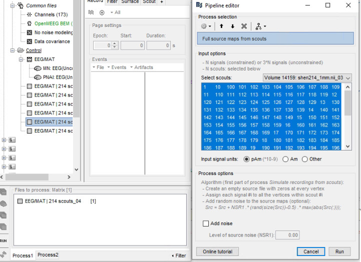
I have been going through the code and in this loop in the function "process_simulate_recordings":

        for i = 1:length(sScouts)
            % Get source indices
            iSourceRows = bst_convert_indices(sScouts(i).Vertices, nComponents, HeadModelMat.GridAtlas, ~isVolumeAtlas);
            % Constrained models: One scout x One signal
            if (nComponents == 1)   
                % Replicate signal values for all the dipoles in the scout
                ImageGridAmp(iSourceRows,:) = repmat(sMatrix.Value(i,:), length(iSourceRows), 1);
            % Unconstrained models: One scout x One orientation (x,y,z) = one signal
            elseif (nComponents == 3)
                for dim = 1:3
                    iSignal = 3*(i-1) + dim;
                    % Replicate signal values for all the dipoles in the scout (with <dim> orientation only)
                    ImageGridAmp(iSourceRows(dim:3:end),:) = repmat(sMatrix.Value(iSignal,:), length(iSourceRows)/3, 1);
                end
            end
        end

This line takes aproximately 45 seconds to compute each time:

% Replicate signal values for all the dipoles in the scout (with <dim> orientation only)
ImageGridAmp(iSourceRows(dim:3:end),:) = repmat(sMatrix.Value(iSignal,:), length(iSourceRows)/3, 1);

So by my rough estimate, it should take Matlab 8 hours to finish this loop, is this normal behavior?

This line takes aproximately 45 seconds to compute each time

This should take a fraction of seconds, unless your signals are very long.

How long are these signals?
If the data you manipulate is too long for your computer, this would pack your memory and make it extremely slow. Try working with shorter blocks of data.

Hi!

Thank you very much. I'm a colleague of @KaizerChef wirking on the same data. The signal is 150k samples long, and the computer is quite powerful (is an instance from a Processing Cluster). Do you think it is considered a "long" signal?

It has been computing for about 36 hours and it has not finished yet....

The signal is 150k samples long

Yes, this is too long:
150000 time samples * 45000 dipoles * 8 bytes = 50 Gb.
It probably needs two copies of this data at some point in memory, so count that it requires 100 Gb of RAM + 50 Gb on the hard drive. It's even surprising that it doesn't crash, you do have some heavy duty computers.

You definitely need to proceed in a different way.
You probably don't need the full length data at the full source-level resolution.
What is your goal exactly?

I see, thank you very much! So, do you think that segmenting the data into 10 second epochs and simulating the sources for each one would be an appropriate approach? We intend to analyse this data with mostly window-based measures, but at some point we would like to do dynamic functional connectivity analyses, so that's why we tried to do this on the full recordings, in order to prevent discontinuities between segments.

I would also like to ask, when we did this process in the non-recommended way ("Downsample to atlas") we didn't run into this problem (or at least I don't recall this). Are these processess fundamentally different?

So, do you think that segmenting the data into 10 second epochs and simulating the sources for each one would be an appropriate approach?

Splitting the EEG recordings would require less memory at once, but it would still save 50Gb of data on the hard drive.

I don't understand this "simulation" logic you are using. If you just use the sources you estimated from the EEG, the source file are saved in an optimized way (ImagingKernel) and then it is very light in terms of storage on the hard drive.
However, when using this file as the input for connectivity analysis, it would still need to reconstruct the full source matrix in memory, and it would probably require hundreds of Gb of RAM. Splitting the EEG data in shorter blocks in this case.

I think you should do your connectivity analysis on the scout signals (214 x 150000). Mapping this on the full cortex would be of no help.

I would also like to ask, when we did this process in the non-recommended way ("Downsample to atlas") we didn't run into this problem (or at least I don't recall this). Are these processess fundamentally different?

The process "Downsample to atlas" extracts the scouts time series (214 x 150000), and saves this as a source file. It does not map the values to each of the 45000 dipoles. Therefore, yes, this is completely different. However, this type of compact storage is not supported by many processes, you can't use this as the input for connectivity processes.

This process was a clumsy attempt to handle scout times series. It is now replaced by the two successive processes "Extract scout time series" and "Full source map from scouts", which allow a lot more flexibility in data processing and display, at the cost of some more manipulation.

First of all, thank you for your reply and your valuable time. We really appreciate it. I think that we almost have it, but we may have mixed some concepts. For simplicity let's consider that we have constraindes sources, thus having only 15000 dipoles:

1. We can directly obtain the source time courses using, "Compute Sources"->sLORETA method. In this case, we can obtain 15000sourcesX150000timeSamples matrices, using "ImgaingKernel" and the original signals.
2. Similarly, we can obtain the scout (i.e., ROI) time courses vía "Downsample To Atlas". In this case we have (if using Desikan-Killiany Atlas) 68scoutsX150000timeSamples
3. The results in point "2" can be also obtained in another way: "Extract"->"Scout Time Series". Is this correct? Is there any difference between results in "2" and "3" (I can see that the icon associated to both results are different)?
4. Finally, by using "Simulate"->"Full Source Maps From Scouts", what do we exactly obtain? The same that in point "1"?

The process "Downsample to atlas" extracts the scouts time series (214 x 150000), and saves this as a source file. It does not map the values to each of the 45000 dipoles. Therefore, yes, this is completely different. However, this type of compact storage is not supported by many processes, you can't use this as the input for connectivity processes.

You mean that Brainstorm can't manage "Source" files for connectivity, right? I mean, the issue is in the format not in the signals themself, and thus I can't use them in my own connectivity pipelines, right?

Thank you again @Francois

The signals stored in the file should be the same, but the container is different and Brainstorm would allow completely different things with each file.
The "source" version (option 2) might not be handled correctly in many processes. It is therefore not recommended, and is going to be removed from the interface at some point.
In general, do not use anything in Brainstorm that is "not recommended" unless you know exactly what you are doing or that you want to reproduce older results that used the deprecated function.

4. Finally, by using "Simulate"->"Full Source Maps From Scouts", what do we exactly obtain? The same that in point "1"?

No. You get the signals or 2) and 3), copied back into a full cortex file. If a scout includes 200 vertices, its time series would be replicated for each of the 200 vertices (= copied to the 200 corresponding rows in ImageGridAmp).

You mean that Brainstorm can't manage "Source" files for connectivity, right?

The connectivity functions handle source files correctly, but not these hacky source files generated with the process "Downsample to atlas".
If you use scouts, it means that you are interested in only e.g. 68 ROI time series, and not the full 15000 source time series. Therefore, you should run your connectivity analyses on these 68 signals, instead of reconstructing and artificial file with 15000 signals, that would later be shrunk again to 68.

Okay! Now I understand!

Thank you very much @Francois