|
Size: 9886
Comment:
|
Size: 13353
Comment:
|
| Deletions are marked like this. | Additions are marked like this. |
| Line 1: | Line 1: |
| = Export source maps to SPM8 = The statistical analysis is still limited in Brainstorm, but you can easily export your source maps and run your tests with an external application. This tutorial explains how to export source maps to SPM8. It is based on the median nerve tutorial dataset that was used in the tutorials of the section [[Tutorials/TutRawViewer|Processing continuous recordings]]. If you have followed those tutorials, this dataset should be available in your database in the protocol '''!TutorialRaw'''. |
= Export volume source maps to SPM8 / SPM12 = The statistical analysis is still limited in Brainstorm, but you can easily export your source maps and run your tests with an external application. This tutorial explains how to export source results to SPM8 or SPM12. The screen captures are done using SPM8, but everything is applicable to SPM12 as well. It is based on the median nerve tutorial dataset that was used in the tutorials of the section [[Tutorials/TutRawViewer|Processing continuous recordings]]. If you have followed those tutorials, this dataset should be available in your database in the protocol '''!TutorialRaw'''. |
| Line 4: | Line 4: |
| SPM8 has an important limitation with respect with SPM12: it cannot work on surfaces. We have to export all the sources to full volumes, which is highly inefficient. If you get the option, consider updating to SPM12. | SPM8 has an important limitation with respect with SPM12: it cannot work on surfaces. This tutorial illustrates how to export all the source files to full volumes. If you are interested in processing the source information at the surface level, upgrade to SPM12 and follow the tutorial [[ExportSpm12|Export surface source maps to SPM12]]. |
| Line 8: | Line 8: |
| == Calculate unconstrained sources == In the previous tutorial, we have calculated sources constrained to the cortex surface. Because SPM8 works only with full volumes, we are going to estimate the sources in the full head volume, as detailed in the tutorial [[Tutorials/TutVolSource|Volume source estimation]]. |
== Export source files == We want to export the sources estimated for all the trials for the '''left '''condition to volume files in NIfTI1 format (readable by SPM). We are going to get rid of the time information, very difficult to handle with those full volumes in SPM, and keep only two averaged time windows per condition: a baseline '''[-20,-15]ms''' and an active state '''[33,38]ms'''. |
| Line 11: | Line 11: |
| Right-click on (common files) > Compute head model > MRI volume. | Clear the Process1 box and drop all the trials for condition Left in it. Select the button "Process sources" on the left of the Process1 tab. |
| Line 13: | Line 13: |
| {{attachment:unconstrHeadmodel.gif||height="239",width="432"}} | {{attachment:introBst.gif||height="364",width="438"}} |
| Line 15: | Line 15: |
| Right-click on the new head model > Compute sources > keep all the default options. | Select the process "File > Export to SPM8 (volume)". |
| Line 17: | Line 17: |
| {{attachment:unconstrSources.gif||height="227",width="387"}} Pick any of the unconstrained source file and drop it in the Process1 box. Run the process "Standardize > Z-score (dynamic)". It creates a new shared source file, available for all the files of Subject01. {{attachment:zscored.gif||height="259",width="473"}} == Export source files == We want now to export the z-scored unconstrained sources to volume files in NIfTI1 format (readable by SPM). We are going to get rid of the time information, very difficult to handle with those full volumes in SPM, and keep only two averaged time windows per condition: a baseline [-20,-15]ms and an active state [33,38]ms. We are going to generate 2*101 left + 2*98 right .nii files. Clear the Process1 box and drop all the trials for condition Left in it. Select the button "Process sources" on the left of the Process1 tab. To select only the unconstrained/z-scored files, you could simply use the checkbox "zscore", but we are going to illustrate a more generic solution: select the process "File > Select files with tag" (detailed in the tutorial [[SelectFiles|Selecting files in the database]]). Configure it as following: {{attachment:selectFiles.gif||height="307",width="478"}} Then in the same pipeline, select the process "File > Export to SPM". {{attachment:exportLeftBaseline.gif||height="319",width="307"}} |
{{attachment:exportLeftBaseline.gif||height="379",width="292"}} |
| Line 36: | Line 21: |
| * '''Output folder''': Select the folder where you want all the .nii files to be saved * '''Output file tag''': Set the file name to this exported .nii files. If you leave this option empty, the default file names would be "Subject01_Left_*.nii", which is not informative enough, given that we want to export two states for the same condition: baseline vs. active. |
* '''Output folder''': Select the file format of the output files (choose "NIfTI-1 (*.nii)"), the select the folder where you want all the .nii files to be saved. * '''Output file tag''': Set the file name of the exported .nii files. If you leave this option empty, the default file names are "!SubjectName_Condition_*.nii", which in this case would be "Subject01_Left_*.nii". This is not informative enough, given that we want to export two states for the same condition: baseline vs. active. Set this option it manually to "subject01_left_baseline". * '''Save all the trials in one file''': If selected, all the trials are concatenated along the "time" dimension in the saved in the same NIfTI file. This is preferable in our case, as we are not planning to use the time dimension: it will generate one file with 101 volumes instead of 101 files containing one volume each. |
| Line 40: | Line 26: |
| * '''Volume downsample''': Set it to 3, it will take one voxel every three voxels in each dimension. The MRI volume we imported in the Brainstorm database is 256x256x256, the output volumes with the functional data are only 86x86x86, again to limit the size of the files we generate at this step. | |
| Line 42: | Line 27: |
| * '''Volume downsample''': Set it to 2, it will take one voxel every two voxels in each dimension. The MRI volume we imported in the Brainstorm database is 256x256x256, the output volumes with the functional data are only 128x128x128, again to limit the size of the files we generate at this step. * '''Use absolute values of the sources''': If this option is selected, the source amplitudes will be all positive instead of positive and negative. This is usually a better way to represent the activation of a brain area, and better adapted for statistical analysis in SPM. * '''Cut empty slices''': If this option is selected, only the slices of the MRI that contain non-zero values are exported in the .nii files. This decreases significantly the output file size, and works well this SPM. |
|
| Line 43: | Line 31: |
| Add another export process right after this one, to export the "active" state. Set the time window to [33,38]ms, to capture the peak of the response in the primary somatosensory cortex, and the file name to "subject01_left_active". | Add another export process after this one, to export the "active" state. Set the time window to [33,38]ms, to capture the peak of the response in the primary somatosensory cortex, and the file name to "subject01_left_active". |
| Line 45: | Line 33: |
| {{attachment:exportLeftActive.gif||height="343",width="309"}} | {{attachment:exportLeftActive.gif||height="391",width="285"}} |
| Line 47: | Line 35: |
| Click on Run and let it process for a while. It will generate 2*101=202 NIfTI files in the output folder. | Click on Run and let it process for a while. It will generate two NIfTI files of 130Mb each in the output folder: '''subject01_left_active.nii''' and '''subject01_left_baseline.nii'''. Each file contains 101 volumes, one per trial. |
| Line 49: | Line 37: |
| Repeat the operation for the right condition: change only the file output names to "subject01_right_baseline" and "subject01_right_active". | You can try opening some of those volumes with a NIfTI file viewer, just to make sure that what is saved is coherent. You can use for instance the free software [[http://www.mccauslandcenter.sc.edu/mricro/mricron/|Mricron]] to view the file subject01_left_active.nii, volume #2. The values saved in this file are not integers, so you may have to edit manually the amplitude scale for the colormap (the text boxes in the second line of toolbar). For instance, set this range from '''0 to 5e-10''' pAm. |
| Line 51: | Line 39: |
| {{attachment:exportRightActive.gif||height="344",width="309"}} | This is a stimulation of the left median nerve, we observe as expected a response in the central regions of the right hemisphere. |
| Line 53: | Line 41: |
| Open you file explorer and check the .nii files that were created in the destination folder. {{attachment:allNii.gif}} You can try opening some of those files with a NIfTI file viewer, just to make sure that what is saved is coherent. You can use for instance the free software [[http://www.mccauslandcenter.sc.edu/mricro/mricron/|Mricron]] to view the file subject01_right_active_02.nii. This a stimulation of the right median nerve, we can see clearly that the response is located in the central regions of the left hemisphere, which is what we expect. {{attachment:mriCron.gif||height="342",width="286"}} Note that you can also you Brainstorm as a NIfTI viewer: go to the anatomy view of the protocol, right-click on Subject01 > Import MRI > Select a .nii file. |
{{attachment:mriCronConstr.gif||height="357",width="292"}} |
| Line 64: | Line 44: |
| One last thing we need to export from Brainstorm: the T1 MRI volume of the subject, on which we would like to see the results in SPM. Go the anatomy view of the protocol !TutorialRaw, right click on Subject01 / MRI > File > Export to file. Select the file format "MRI: NIfTI-1" and save the file '''T1.nii''' in the same folder with all the other .nii files. | One last thing you need to export from Brainstorm: the T1 MRI volume of the subject, for displaying the results in SPM. Go the anatomy view of the protocol !TutorialRaw, right click on Subject01 / MRI > File > Export to file. Select the file format "MRI: NIfTI-1" and save the file '''T1.nii''' in the same folder with all the other .nii files. |
| Line 72: | Line 52: |
'''Import note''': Do not run Brainstorm and SPM at the same time, always close Brainstorm before starting SPM (but you don't need to close Matlab). |
|
| Line 81: | Line 63: |
| * '''Directory''': Select the folder in which the results to be saved, for instance create a sub-folder "spm" in the folder in which you have saved all the NIfTI files. | * '''Directory''': Select the folder in which the results to be saved, for instance create a sub-folder "spm" in the folder in which you have saved all the NIfTI files (see following note) |
| Line 83: | Line 65: |
| * '''Group 1 scans''': Select all the post-stim trials for the left condition (subject01_left_active_*.nii) * '''Group 2 scans''': Select all the pre-stim trials for the left condition (subject01_left_baseline_*.nii) |
* '''Group 1 scans''': Select the 101 post-stim trials, from file '''subject01_left_active.nii''' (see note) * '''Group 2 scans''': Select the 101 pre-stim trials, from file '''subject01_left_baseline.nii''' (see note) |
| Line 90: | Line 72: |
| '''(*) File selector''': Using the SPM file selector for importing the 4D NIfTI files we have exported from Brainstorm is not that intuitive. Follow those guidelines: * Navigate to select the folder containing your two .nii files using the two lists on the top (Up,Prev) and the LEFT directory list * Edit the selected volumes in the text box containing only a "1", replace it with "'''1:999'''" . This will display all the volumes from 1 to 999 in the RIGHT file list * Click on a file in the RIGHT file list to select it: it is removed from the right list and added to the bottom list (selected files) * You can then scroll down, hold the shift key and click on the last file you want to select, to add all the entries in between. * If you made a mistake and want to unselect a file: just click on it in the bottom list, it will go back to the right file list. * Click on "Done" when the 101 trials are selected {{attachment:spmFileSelect.gif||height="327",width="412"}} Once you have defined all the options, click on the '''Run '''button (the green button in the toolbar on top of the Batch Editor window). |
|
| Line 92: | Line 87: |
| Once you have defined all the options, click on the '''Run '''button (the green button in the toolbar on top of the Batch Editor window). The design matrix window is displayed in the Graphics window, and a file SPM.mat is saved in the output directory you defined in the options. | The design matrix window is displayed in the Graphics window, and a file '''SPM.mat''' is saved in the output directory you defined in the options. |
| Line 96: | Line 91: |
| In the SPM8 Menu window, click on the '''Estimate''' button. Select the SPM.mat file that was just created. SPM estimates the parameters, it may take a while. | In the SPM Menu window, click on the '''Estimate''' button. Select the '''SPM.mat''' file that was just created. SPM estimates the parameters, it may take a while. |
| Line 100: | Line 95: |
| When done click on '''Results''' in the SPM8 Menu window, select again the same SPM.mat file. A window pops up, you have to specify the contrast(s) of interest. | When done click on '''Results''' in the SPM Menu window, select again the same '''SPM.mat''' file. A window pops up, you have to specify the contrast(s) of interest. |
| Line 104: | Line 99: |
| Click on "Define new constrast...". Edit the options to define the t-test post-stim > pre-stim: | Click on "Define new contrast...". Edit the options to define the t-test post-stim > pre-stim: |
| Line 107: | Line 102: |
| * '''Type''': t-constrast | * '''Type''': t-contrast |
| Line 117: | Line 112: |
| Click on "Done", then a list of parameters is asked in the "SPM8: Stats: Results" window. | Click on "Done", then a list of parameters is asked in the "SPM: Stats: Results" window. |
| Line 122: | Line 117: |
| * '''p-value (FWE)''': 0.05 | * '''p-value (FWE)''': 0.01 |
| Line 126: | Line 121: |
| {{attachment:spmContrast4.gif||height="224",width="308"}} | {{attachment:spmContrast4.gif||height="335",width="324"}} |
| Line 128: | Line 123: |
| Then the typical SPM8 glass brain shows up in the Graphics window. The window SPM8 Results shows more display options for this figure. Select "'''overlays > sections'''". Pick the file '''T1.nii''' we exported from Brainstorm. | Then the typical SPM glass brain shows up in the Graphics window. The results don't look nicely aligned on this view because the source volumes have not been normalized to the MNI brain. If you are interested in projecting your sources in the MNI space, we recommend you do it from Brainstorm directly. The concept and procedure are explained in the tutorial [[Tutorials/CoregisterSubjects|Group studies: Subject coregistration]]. |
| Line 130: | Line 125: |
| {{attachment:spmContrast5.gif||height="214",width="327"}} | The window SPM Results shows more display options for this figure. Select "'''overlays > sections'''". Pick the file '''T1.nii''' you exported from Brainstorm. {{attachment:spmContrast5.gif||height="352",width="323"}} |
| Line 134: | Line 131: |
| {{attachment:spmResults.gif||height="461",width="307"}} | {{attachment:spmResultsConstr.gif||height="581",width="388"}} |
| Line 140: | Line 137: |
| == Clean Brainstorm database == To restore the original state of the protocol !TutorialRaw and be able to use it as the starting point for another advanced tutorial, delete the three new files in Subject01 / Common files: |
== Using unconstrained sources == We have done this analysis using a source model where all the dipoles where located in the grey matter, with orientations constrained to the normal of the cortex surface. You can repeat the same analysis using sources distributed in the full brain volume, as detailed in the tutorial [[http://neuroimage.usc.edu/brainstorm/Tutorials/TutVolSource|Volume source estimation]]. Right-click on (common files) > Compute head model > MRI volume. Use the default options for the grid of points. {{attachment:unconstrHeadmodel.gif|height="239",width="432"|height="225",width="407"}} Right-click on the new head model > Compute sources > keep all the default options. {{attachment:unconstrSources.gif|height="227",width="387"|height="235",width="401"}} We want now to export the unconstrained sources to volume files in NIfTI1 format. Clear the Process1 box and drop all the trials for condition Left in it. Select the button "Process sources" on the left of the Process1 tab. Problem: it selects at the same time the constrained and unconstrained sources (total 202 files instead of 101). We can use the process "File > Select files with tag" (detailed in the tutorial [[http://neuroimage.usc.edu/brainstorm/SelectFiles|Selecting files in the database]]). Configure it as following: {{http://neuroimage.usc.edu/brainstorm/ExportSpm8?action=AttachFile&do=get&target=selectFiles.gif|selectFiles.gif|height="307",width="478",class="attachment"}} Add immediately after the two processes to export the baseline and the active state (use a different folder). Set the same options as previous (constrained case). Then click on Run. {{attachment:exportUnconstr.gif||height="399",width="276"}} Look for instance at the file subject01_left_active.nii, volume #2, [0 2e-10] pAm. {{attachment:mriCron.gif||height="363",width="277"}} Close Brainstorm, start SPM, and run exactly the same analysis steps as before. In the end you should obtain the following results. {{attachment:spmResults.gif||height="560",width="375"}} === Clean Brainstorm database === To restore the original state of the protocol !TutorialRaw and be able to use it as the starting point for another advanced tutorial, delete the two new files in Subject01 / Common files: |
| Line 145: | Line 171: |
| * MN: MEG(Unconstr) | abs | zscored | |
| Line 147: | Line 172: |
| {{attachment:restoreDb.gif||height="270",width="306"}} | {{attachment:restoreDb.gif||height="299",width="283"}} |
Export volume source maps to SPM8 / SPM12
The statistical analysis is still limited in Brainstorm, but you can easily export your source maps and run your tests with an external application. This tutorial explains how to export source results to SPM8 or SPM12. The screen captures are done using SPM8, but everything is applicable to SPM12 as well. It is based on the median nerve tutorial dataset that was used in the tutorials of the section ?Processing continuous recordings. If you have followed those tutorials, this dataset should be available in your database in the protocol TutorialRaw.
SPM8 has an important limitation with respect with SPM12: it cannot work on surfaces. This tutorial illustrates how to export all the source files to full volumes. If you are interested in processing the source information at the surface level, upgrade to SPM12 and follow the tutorial Export surface source maps to SPM12.
Export source files
We want to export the sources estimated for all the trials for the left condition to volume files in NIfTI1 format (readable by SPM). We are going to get rid of the time information, very difficult to handle with those full volumes in SPM, and keep only two averaged time windows per condition: a baseline [-20,-15]ms and an active state [33,38]ms.
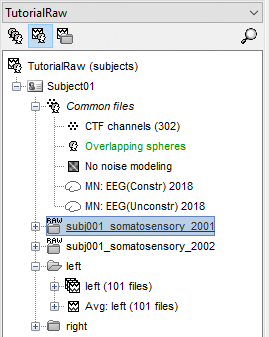
Clear the Process1 box and drop all the trials for condition Left in it. Select the button "Process sources" on the left of the Process1 tab.
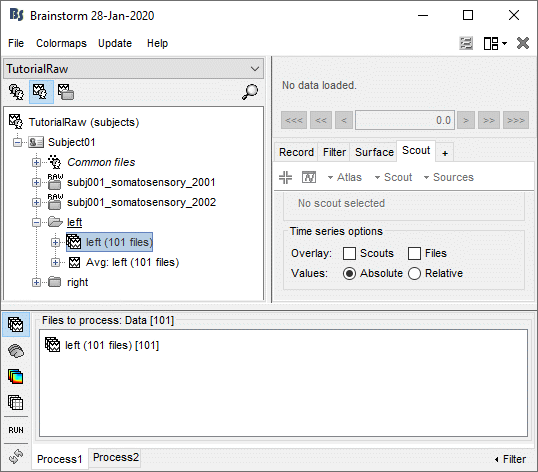
Select the process "File > Export to SPM8 (volume)".
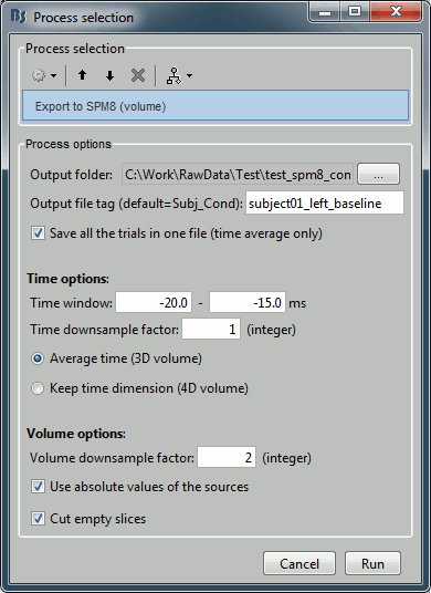
Configure the process:
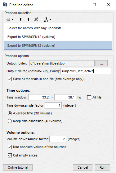
Output folder: Select the file format of the output files (choose "NIfTI-1 (*.nii)"), the select the folder where you want all the .nii files to be saved.
Output file tag: Set the file name of the exported .nii files. If you leave this option empty, the default file names are "SubjectName_Condition_*.nii", which in this case would be "Subject01_Left_*.nii". This is not informative enough, given that we want to export two states for the same condition: baseline vs. active. Set this option it manually to "subject01_left_baseline".
Save all the trials in one file: If selected, all the trials are concatenated along the "time" dimension in the saved in the same NIfTI file. This is preferable in our case, as we are not planning to use the time dimension: it will generate one file with 101 volumes instead of 101 files containing one volume each.
Time window: Segment of the file that we want to export. We start with the baseline: -20ms to -15ms
Time downsample factor: If we keep the time information, we can save only one time sample every N in the .nii files, to limit the size of the generated files. The value we set here is not used because we specify in the last option that we average in the time dimension.
Average over time / Keep time dimension: Defines what we do with the time. In this case, we want to average over the small time windows to get rid of the time.
Volume downsample: Set it to 2, it will take one voxel every two voxels in each dimension. The MRI volume we imported in the Brainstorm database is 256x256x256, the output volumes with the functional data are only 128x128x128, again to limit the size of the files we generate at this step.
Use absolute values of the sources: If this option is selected, the source amplitudes will be all positive instead of positive and negative. This is usually a better way to represent the activation of a brain area, and better adapted for statistical analysis in SPM.
Cut empty slices: If this option is selected, only the slices of the MRI that contain non-zero values are exported in the .nii files. This decreases significantly the output file size, and works well this SPM.
Add another export process after this one, to export the "active" state. Set the time window to [33,38]ms, to capture the peak of the response in the primary somatosensory cortex, and the file name to "subject01_left_active".
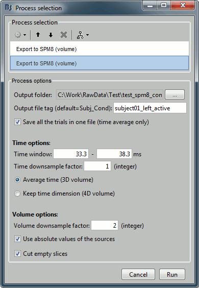
Click on Run and let it process for a while. It will generate two NIfTI files of 130Mb each in the output folder: subject01_left_active.nii and subject01_left_baseline.nii. Each file contains 101 volumes, one per trial.
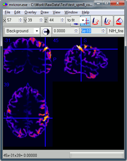
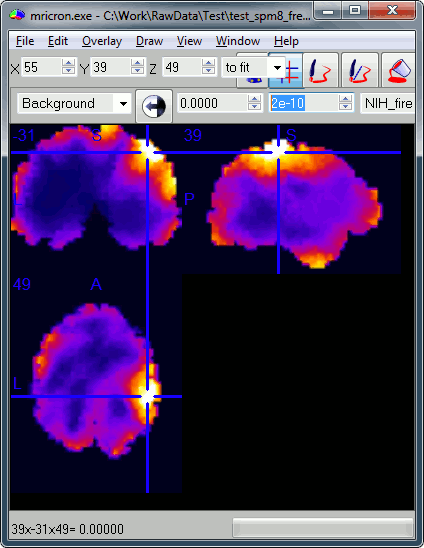
You can try opening some of those volumes with a NIfTI file viewer, just to make sure that what is saved is coherent. You can use for instance the free software Mricron to view the file subject01_left_active.nii, volume #2. The values saved in this file are not integers, so you may have to edit manually the amplitude scale for the colormap (the text boxes in the second line of toolbar). For instance, set this range from 0 to 5e-10 pAm.
This is a stimulation of the left median nerve, we observe as expected a response in the central regions of the right hemisphere.
Export T1 MRI
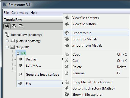
One last thing you need to export from Brainstorm: the T1 MRI volume of the subject, for displaying the results in SPM. Go the anatomy view of the protocol TutorialRaw, right click on Subject01 / MRI > File > Export to file. Select the file format "MRI: NIfTI-1" and save the file T1.nii in the same folder with all the other .nii files.
Run SPM
Installing SPM is easy: http://www.fil.ion.ucl.ac.uk/spm/software/spm8/
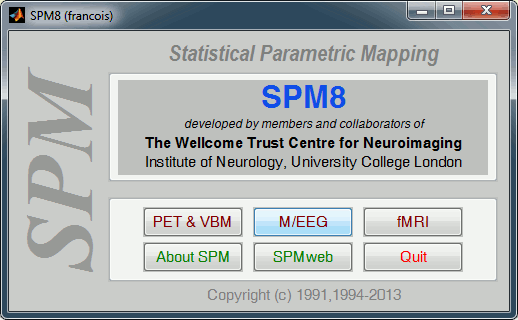
Start Matlab, go to the SPM folder, add it to your path if it is not done already, then type "spm". Select "M/EEG" on the SPM startup screen.
Import note: Do not run Brainstorm and SPM at the same time, always close Brainstorm before starting SPM (but you don't need to close Matlab).
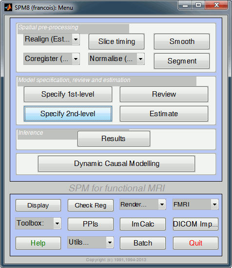
In the main SPM window, click on "Specify 2nd level".
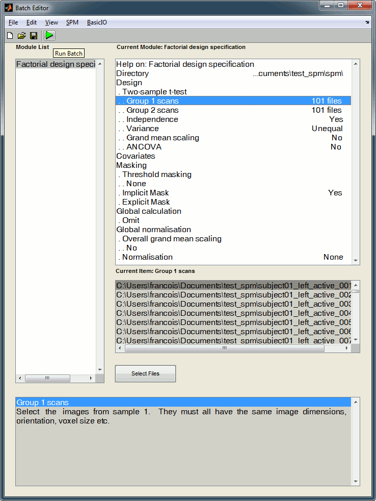
Now you can specify your stats design in the Batch Editor window. We are going to start with a simple t-test for the left condition: active state versus baseline. Select the following options:
Directory: Select the folder in which the results to be saved, for instance create a sub-folder "spm" in the folder in which you have saved all the NIfTI files (see following note)
Design: Two sample t-test
Group 1 scans: Select the 101 post-stim trials, from file subject01_left_active.nii (see note)
Group 2 scans: Select the 101 pre-stim trials, from file subject01_left_baseline.nii (see note)
Independence: Yes
Variance: Unequal
Grand mean scaling: No
ANCOVA: No
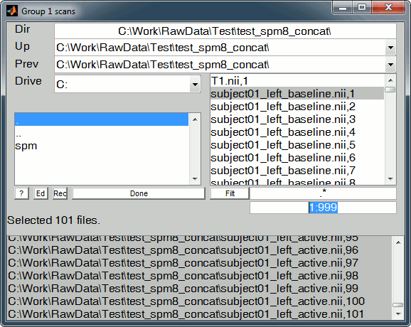
(*) File selector: Using the SPM file selector for importing the 4D NIfTI files we have exported from Brainstorm is not that intuitive. Follow those guidelines:
- Navigate to select the folder containing your two .nii files using the two lists on the top (Up,Prev) and the LEFT directory list
Edit the selected volumes in the text box containing only a "1", replace it with "1:999" . This will display all the volumes from 1 to 999 in the RIGHT file list
- Click on a file in the RIGHT file list to select it: it is removed from the right list and added to the bottom list (selected files)
- You can then scroll down, hold the shift key and click on the last file you want to select, to add all the entries in between.
- If you made a mistake and want to unselect a file: just click on it in the bottom list, it will go back to the right file list.
- Click on "Done" when the 101 trials are selected
Once you have defined all the options, click on the Run button (the green button in the toolbar on top of the Batch Editor window).
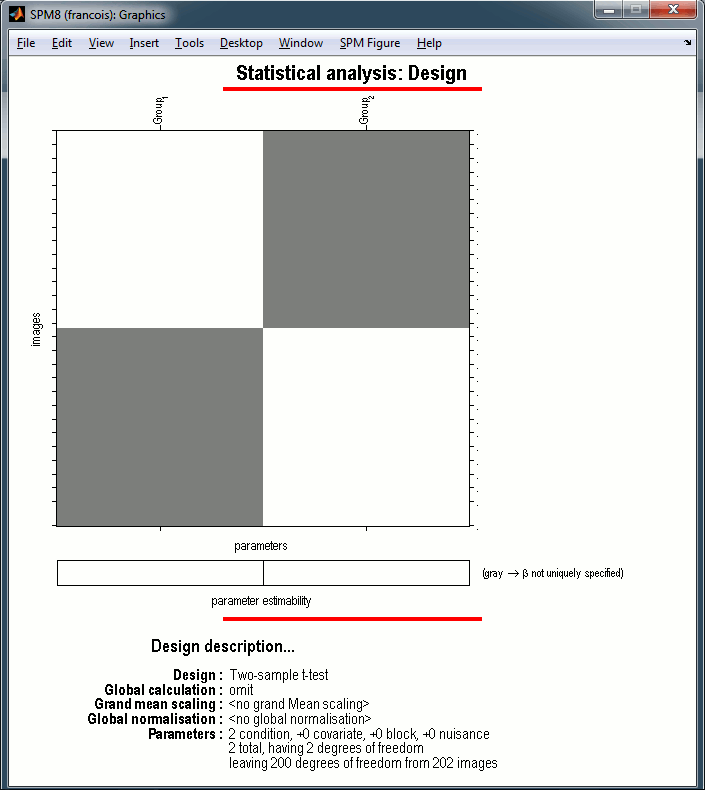
The design matrix window is displayed in the Graphics window, and a file SPM.mat is saved in the output directory you defined in the options.
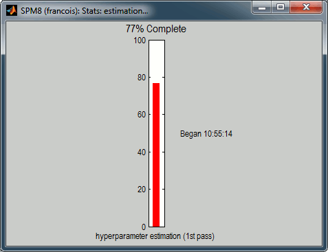
In the SPM Menu window, click on the Estimate button. Select the SPM.mat file that was just created. SPM estimates the parameters, it may take a while.
When done click on Results in the SPM Menu window, select again the same SPM.mat file. A window pops up, you have to specify the contrast(s) of interest.
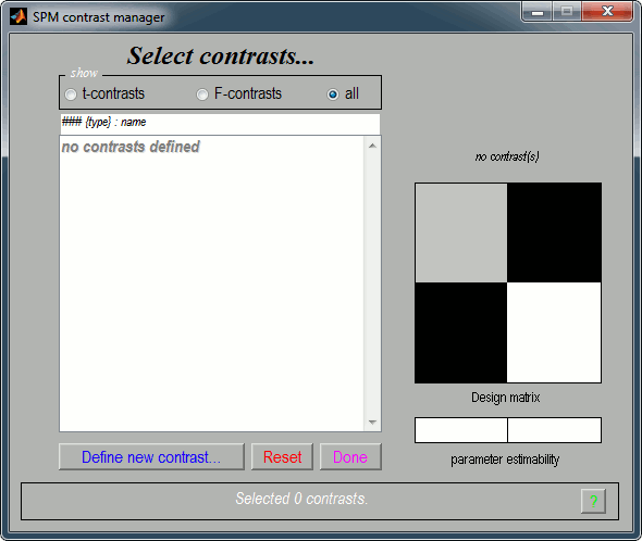
Click on "Define new contrast...". Edit the options to define the t-test post-stim > pre-stim:
Name: Give a name to the contrast, for display. Enter for instance "Active>Baseline".
Type: t-contrast
Contrast: Enter "1 -1" to test for "Group1 (active files) > Group2 (baseline files)"
- Click on "...submit" to update the figure, then "Ok" to add the new contrast.
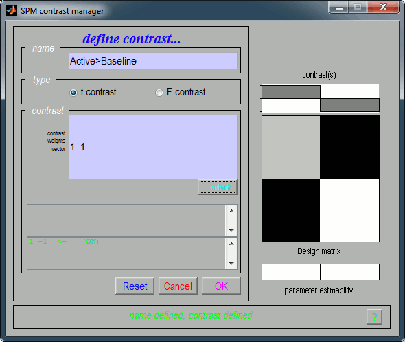
It updates the window "SPM contrast manager".
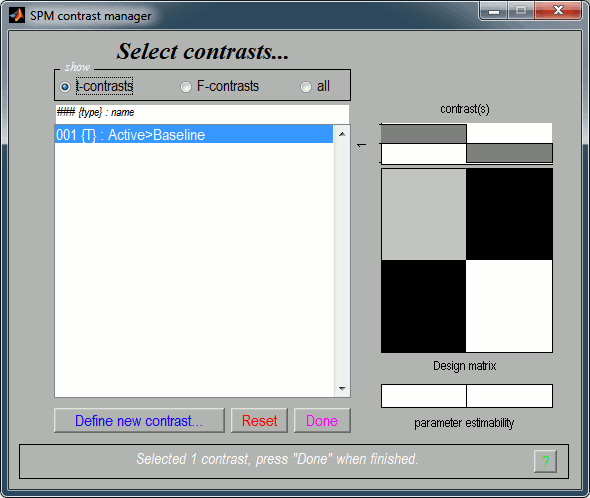
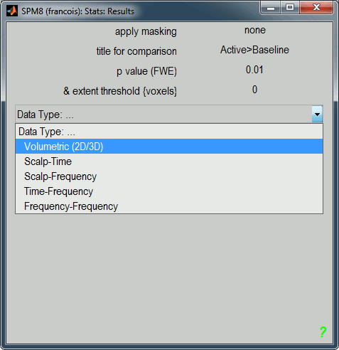
Click on "Done", then a list of parameters is asked in the "SPM: Stats: Results" window.
Apply masking: None
Title for comparison: "Active>Baseline" for instance
p-value adjustment to control: FWE (=Family-Wise Error, to correct for multiple comparisons)
p-value (FWE): 0.01
& extent threshold (voxels): 0
Data type: Volumetric (2D/3D)
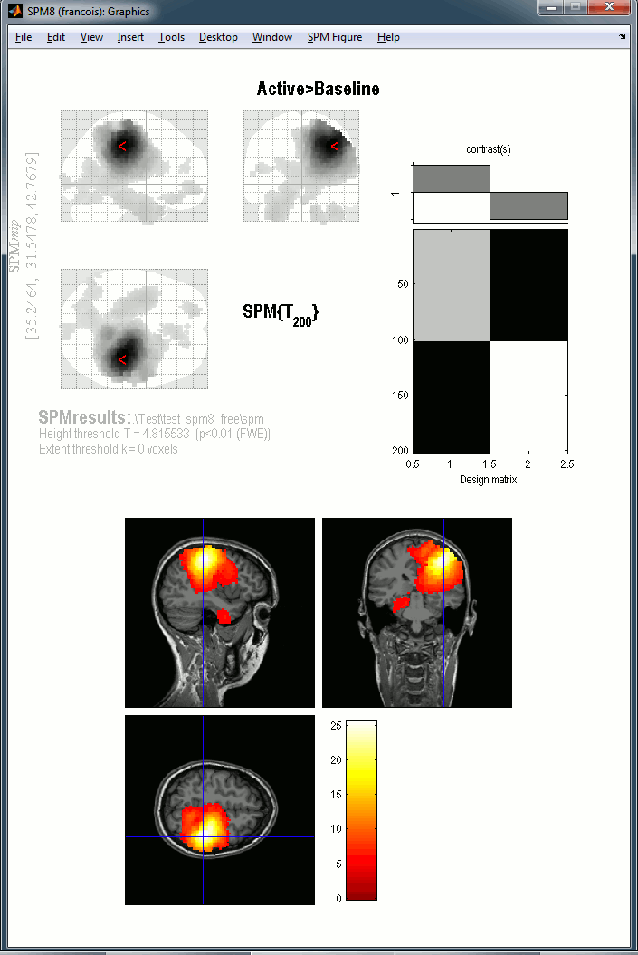
Then the typical SPM glass brain shows up in the Graphics window. The results don't look nicely aligned on this view because the source volumes have not been normalized to the MNI brain. If you are interested in projecting your sources in the MNI space, we recommend you do it from Brainstorm directly. The concept and procedure are explained in the tutorial Group studies: Subject coregistration.
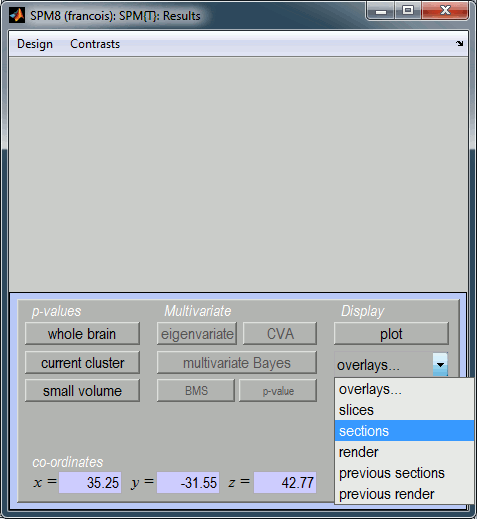
The window SPM Results shows more display options for this figure. Select "overlays > sections". Pick the file T1.nii you exported from Brainstorm.
You get the final results in the Graphics window. You can explore the volume by clicking on the MRI slices.
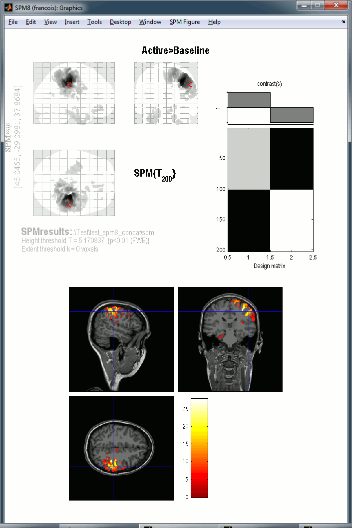
You can repeat the same operations with the right condition.
The results you get here are very basic, but the logic of exporting source results from Brainstorm to SPM can be extended to any type of analysis.
Using unconstrained sources
We have done this analysis using a source model where all the dipoles where located in the grey matter, with orientations constrained to the normal of the cortex surface. You can repeat the same analysis using sources distributed in the full brain volume, as detailed in the tutorial Volume source estimation.
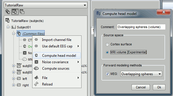
Right-click on (common files) > Compute head model > MRI volume. Use the default options for the grid of points.
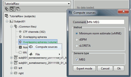
Right-click on the new head model > Compute sources > keep all the default options.
We want now to export the unconstrained sources to volume files in NIfTI1 format. Clear the Process1 box and drop all the trials for condition Left in it. Select the button "Process sources" on the left of the Process1 tab.
Problem: it selects at the same time the constrained and unconstrained sources (total 202 files instead of 101). We can use the process "File > Select files with tag" (detailed in the tutorial Selecting files in the database). Configure it as following:
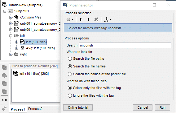
Add immediately after the two processes to export the baseline and the active state (use a different folder). Set the same options as previous (constrained case). Then click on Run.
Look for instance at the file subject01_left_active.nii, volume #2, [0 2e-10] pAm.
Close Brainstorm, start SPM, and run exactly the same analysis steps as before. In the end you should obtain the following results.
Clean Brainstorm database
To restore the original state of the protocol TutorialRaw and be able to use it as the starting point for another advanced tutorial, delete the two new files in Subject01 / Common files:
- Overlapping spheres (volume)
- MN: MEG(Unconstr)
