|
Size: 576
Comment:
|
Size: 7195
Comment:
|
| Deletions are marked like this. | Additions are marked like this. |
| Line 2: | Line 2: |
| == Featuring MEG auditory evoked responses == Acquisition on an ''Elekta'' ''Neuromag Vectorview306'', instrument. Brief description of the following pictures: * Main Brainstorm window * Time series of all MEG sensors [-200, 500] ms * Magnetic field topographty, magnetometers at t=106ms * Topographical layout of magnetometers time series [-200, 500] ms * Modeling of cortical currents, obtained from magnetometers, at t=106ms [[attachment:snap_1condition.jpg|{{attachment:snap_1condition_sm.jpg|attachment:snap_1condition.jpg}}]] |
|
| Line 4: | Line 17: |
| == Keeping your data organized and accessible == The tree in the main Brainstorm window represents the database for the selected study. This database has three levels of definition: Protocol (ie. study, selected in the toolbar), Subject, and Condition. Most of the operations that can be performed on a file are easily accessible from the popup menu revealed by right-clicking over the file. The first three buttons in the toolbar allows the user to switch between different views of the same database: * Anatomy: display the MRI and surfaces for each participant in the study * Functional data (sorted by subject): sensor definitions, MEG and EEG data, source models, statistic and time-frequency maps * Functional data (sorted by condition): same as above, but sorted in a different way The following example features a MEG+EEG protocol called "''Catching''", sorted by conditions. There are two experimental conditions, ''Catch ''and ''NoCatch'', and 7 subjects per condition. The popup menu shows all the actions that are available for the recordings of subject ''cc'', condition ''Catch''. [[attachment:snap_rightclick.jpg|{{attachment:snap_rightclick_sm.jpg|attachment:snap_rightclick.jpg}}]] |
|
| Line 5: | Line 31: |
| || {{attachment:snap_1condition.jpg||height="373",width="534"}} ||<style="vertical-align: top;">'''MEG auditory evoked potential'''<<BR>> (Neuromag Vectorview306)<<BR>> <<BR>> Description of the windows (left to right): [[MiniPage(* Main BrainStorm window * Timeseries of all the MEG sensors [-200ms, 500ms] * Magnetic field recorded by the magnetometers at t=106ms * Spatial view of the magnetometers time series [-200ms, 500ms] * Reconstruction of the cortical currents, based on the magnetometers, at t=106ms)]] || | |
| Line 7: | Line 32: |
| == Multiple conditions: Baby auditory EEG responses == Acquisition system: ''EGI GSN - Baby 64 electrodes'' |
|
| Line 8: | Line 35: |
| Description: | |
| Line 9: | Line 37: |
| * One subject: "001" * Three conditions: "GM", "GMM", "VM" * Two views: overlaid electrodes time series, and estimated cortical sources at t=376ms |
|
| Line 10: | Line 41: |
| ---- | [[attachment:snap_3conditions.jpg|{{attachment:snap_3conditions_sm.jpg|attachment:snap_3conditions.jpg}}]] |
| Line 12: | Line 44: |
== Subject anatomy: MRI and surfaces == Brainstorm features the possibility to model MEG and EEG neural generators either from the individual subject anatomy, or by using a template anatomy (MNI / Colin27) that can be warped to the individual scalp surface. Multiple interactive tools are available to view, register and process the MR images and the corresponding tessellated envelopes. However, tissue segmentation must be performed using another software; multiple options exist today in the academic community ([[Links|listed here]]). We provide a few examples of the views you can easily obtain with Brainstorm. All the 3D views can be rotated freely with the mouse, zoomed with the wheel, edited with the "Surface panel" and contextual popup menus. The MRI slices can be browsed with a simple mouse operation: right-click and mouse drag. [[attachment:snap_anatomy.jpg|{{attachment:snap_anatomy_sm.jpg|attachment:snap_anatomy.jpg}}]] <<BR>> == Channel selection == All the figures displayed by Brainstorm are linked in time. If they feature the same dataset, the sensor selection is also the same for all views. The selection of a channel subset can be easily perfomed by clicking on the corresponding channels in a time series display or a 3D view. Selected channels can be displayed separately, marked as "bad", or deleted. [[attachment:snap_channel.jpg|{{attachment:snap_channel_sm.jpg|attachment:snap_channel.jpg}}]] <<BR>> == Online bandpass filtering == Recordings and sources: 40Hz low-pass filtering with the "Filters" tab in main Brainstorm window. {{attachment:snap_online_filter.jpg|attachment:snap_online_filter.jpg}} <<BR>> == Defining cortical region of interest: Scout == Acquisition system: ''CTF MEG - 151 sensors'' Scouts are cortical regions of interest, defined graphically from the "Scouts" tab. They can be used to extract the time series of MEG and EEG generators within a single or mulitlple brain region. The following example shows the cortical response to an electric stimulation of the left index finger. With the two scouts ''Left ''and ''Right,'' one can observe the electrical activity in the primary somatosensory cortex from each hemisphere. [[attachment:snap_1scout.jpg|{{attachment:snap_1scout_sm.jpg|attachment:snap_1scout.jpg}}]] <<BR>> == Scouts: browsing through multiple conditions == Acquisition system: ''CTF MEG - 151 sensors'' Same experiment than in the previous example, now showing the responses for two conditions: ''Left-1'' (electric stimulation of the left index finger) and ''Left-4'' (left ring finger). [[attachment:snap_2scouts.jpg|{{attachment:snap_2scouts_sm.jpg|attachment:snap_2scouts.jpg}}]] <<BR>> == From surface to volume: MRI integration == Acquisition system: ''CTF MEG - 151 sensors'' Same experiment as above, with additional 3D display of the scout activity in MRI slices. [[attachment:snap_scout3D.jpg|{{attachment:snap_scout3D_sm.jpg|attachment:snap_scout3D.jpg}}]] <<BR>> == Time-frequency decompositions == Acquisition system: ''CTF MEG - 151 sensors'' Time-frequency decompositions of sensor data and source time series, extracted from cortical regions of interest. [[attachment:snap_timefreq.jpg|{{attachment:snap_timefreq_sm.jpg|attachment:snap_timefreq.jpg}}]] <<BR>> == Standardization: z-score == Acquisition system: ''EGI GSN - Baby 64 electrodes'' The "''Processes''" tab in the main Brainstorm window allows users to apply multiple processes to a set of data or source maps. Just drag and drop files from the database tree to the box in the "Processes" tab, and click on "''Run''" to start the processing. The function that was applied here is a simple z-score standardization. The top-right figure displays the initial sources estimate, and the bottom-left figure shows the corresponding z-score valued source map. [[attachment:snap_zscore.jpg|{{attachment:snap_zscore_sm.jpg|attachment:snap_zscore.jpg}}]] <<BR>> == Statistical inference: t-test maps == Acquisition system: ''EGI GSN - Baby 64 electrodes'' The "''Processes''" tab can also be used for running statistical tests e.g., to evaluate contrasts between two experimental conditions. The following example features the evaluation of the difference between conditions ''GM'' and ''GMM'', from the source maps of mulitple subjects (paired Student t-test, p<0.05). The top figure shows the significance of the difference at the sensor level across time. The bottom figure displays the thresholded t-values at the cortical level at 280ms. This image also illustrates the "''Coordinates''" tab: It is possible to pick any point from any surface by clicking on it, and immediately get its coordinates in all the coordinates systems used by Brainstorm (MRI, Subject's head and Talairach). [[attachment:snap_ttest.jpg|{{attachment:snap_ttest_sm.jpg|attachment:snap_ttest.jpg}}]] <<BR>> |
Screenshots
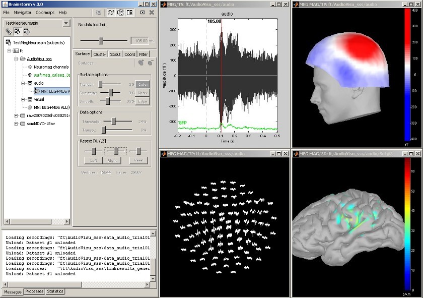
Featuring MEG auditory evoked responses
Acquisition on an Elekta Neuromag Vectorview306, instrument.
Brief description of the following pictures:
- Main Brainstorm window
- Time series of all MEG sensors [-200, 500] ms
- Magnetic field topographty, magnetometers at t=106ms
- Topographical layout of magnetometers time series [-200, 500] ms
- Modeling of cortical currents, obtained from magnetometers, at t=106ms
Keeping your data organized and accessible
The tree in the main Brainstorm window represents the database for the selected study. This database has three levels of definition: Protocol (ie. study, selected in the toolbar), Subject, and Condition. Most of the operations that can be performed on a file are easily accessible from the popup menu revealed by right-clicking over the file.
The first three buttons in the toolbar allows the user to switch between different views of the same database:
- Anatomy: display the MRI and surfaces for each participant in the study
- Functional data (sorted by subject): sensor definitions, MEG and EEG data, source models, statistic and time-frequency maps
- Functional data (sorted by condition): same as above, but sorted in a different way
The following example features a MEG+EEG protocol called "Catching", sorted by conditions. There are two experimental conditions, Catch and NoCatch, and 7 subjects per condition. The popup menu shows all the actions that are available for the recordings of subject cc, condition Catch.
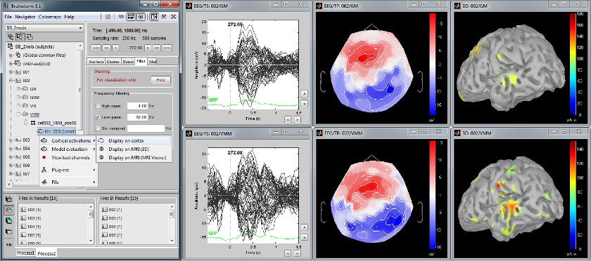
Multiple conditions: Baby auditory EEG responses
Acquisition system: EGI GSN - Baby 64 electrodes
Description:
- One subject: "001"
- Three conditions: "GM", "GMM", "VM"
- Two views: overlaid electrodes time series, and estimated cortical sources at t=376ms
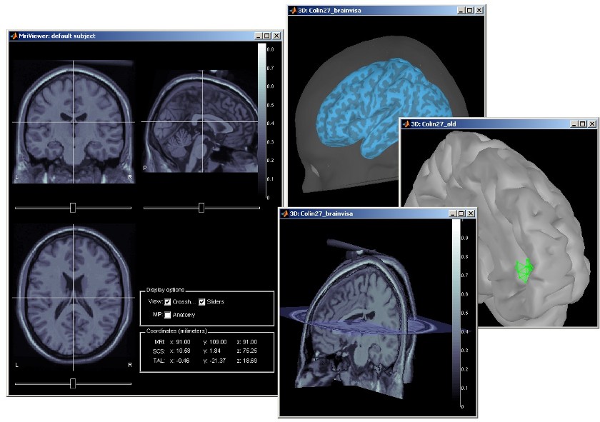
Subject anatomy: MRI and surfaces
Brainstorm features the possibility to model MEG and EEG neural generators either from the individual subject anatomy, or by using a template anatomy (MNI / Colin27) that can be warped to the individual scalp surface. Multiple interactive tools are available to view, register and process the MR images and the corresponding tessellated envelopes. However, tissue segmentation must be performed using another software; multiple options exist today in the academic community (?listed here).
We provide a few examples of the views you can easily obtain with Brainstorm. All the 3D views can be rotated freely with the mouse, zoomed with the wheel, edited with the "Surface panel" and contextual popup menus. The MRI slices can be browsed with a simple mouse operation: right-click and mouse drag.
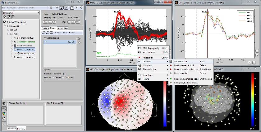
Channel selection
All the figures displayed by Brainstorm are linked in time. If they feature the same dataset, the sensor selection is also the same for all views. The selection of a channel subset can be easily perfomed by clicking on the corresponding channels in a time series display or a 3D view. Selected channels can be displayed separately, marked as "bad", or deleted.
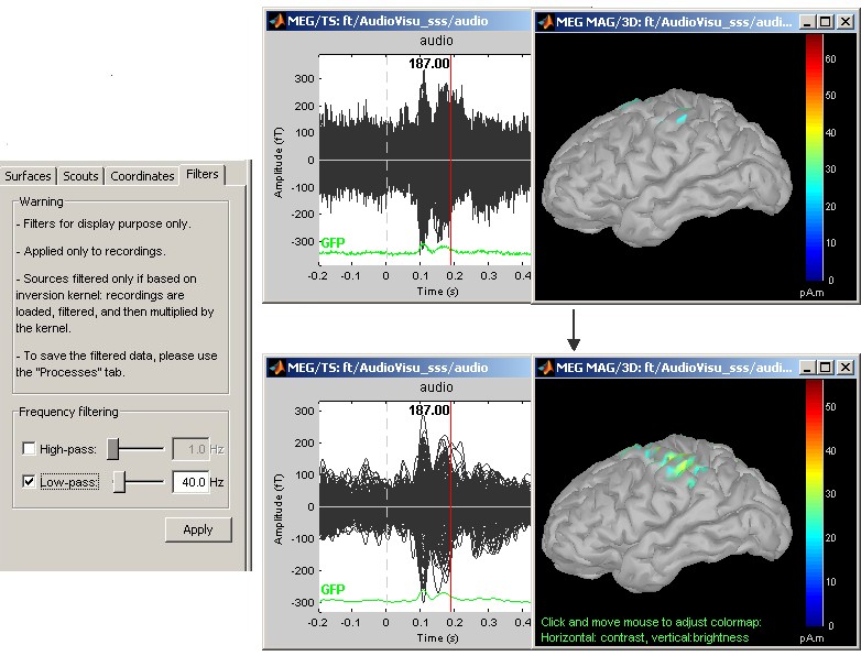
Online bandpass filtering
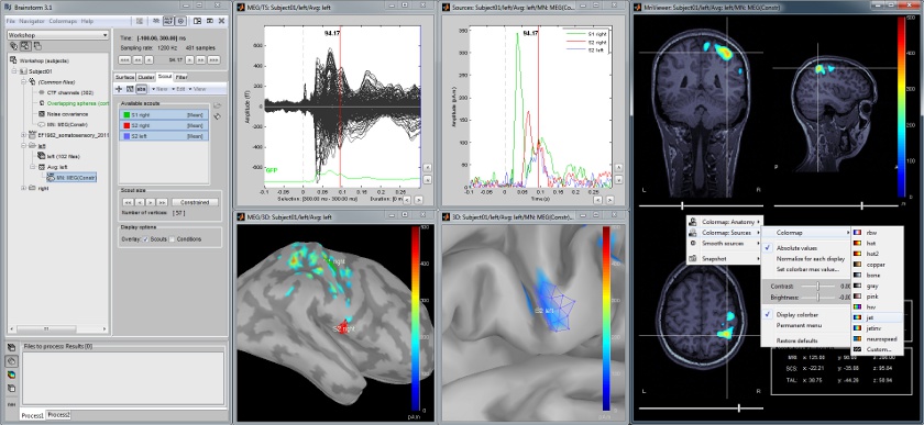
Recordings and sources: 40Hz low-pass filtering with the "Filters" tab in main Brainstorm window.
Defining cortical region of interest: Scout
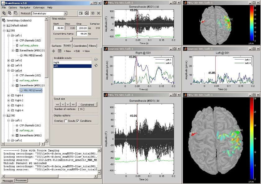
Acquisition system: CTF MEG - 151 sensors
Scouts are cortical regions of interest, defined graphically from the "Scouts" tab. They can be used to extract the time series of MEG and EEG generators within a single or mulitlple brain region.
The following example shows the cortical response to an electric stimulation of the left index finger. With the two scouts Left and Right, one can observe the electrical activity in the primary somatosensory cortex from each hemisphere.
Scouts: browsing through multiple conditions
Acquisition system: CTF MEG - 151 sensors
Same experiment than in the previous example, now showing the responses for two conditions: Left-1 (electric stimulation of the left index finger) and Left-4 (left ring finger).
From surface to volume: MRI integration
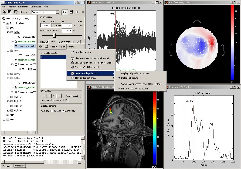
Acquisition system: CTF MEG - 151 sensors
Same experiment as above, with additional 3D display of the scout activity in MRI slices.
Time-frequency decompositions
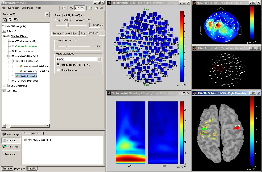
Acquisition system: CTF MEG - 151 sensors
Time-frequency decompositions of sensor data and source time series, extracted from cortical regions of interest.
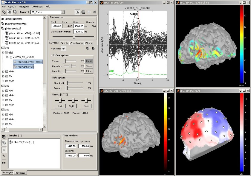
Standardization: z-score
Acquisition system: EGI GSN - Baby 64 electrodes
The "Processes" tab in the main Brainstorm window allows users to apply multiple processes to a set of data or source maps. Just drag and drop files from the database tree to the box in the "Processes" tab, and click on "Run" to start the processing.
The function that was applied here is a simple z-score standardization.
The top-right figure displays the initial sources estimate, and the bottom-left figure shows the corresponding z-score valued source map.
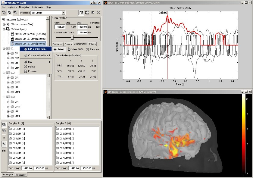
Statistical inference: t-test maps
Acquisition system: EGI GSN - Baby 64 electrodes
The "Processes" tab can also be used for running statistical tests e.g., to evaluate contrasts between two experimental conditions.
The following example features the evaluation of the difference between conditions GM and GMM, from the source maps of mulitple subjects (paired Student t-test, p<0.05). The top figure shows the significance of the difference at the sensor level across time. The bottom figure displays the thresholded t-values at the cortical level at 280ms.
This image also illustrates the "Coordinates" tab: It is possible to pick any point from any surface by clicking on it, and immediately get its coordinates in all the coordinates systems used by Brainstorm (MRI, Subject's head and Talairach).

