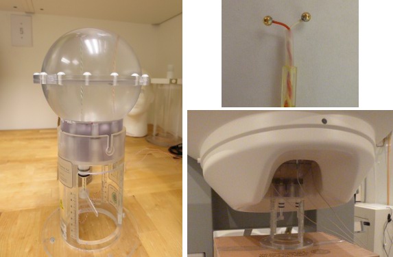
MEG current phantom (CTF)
Authors: Francois Tadel, Elizabeth Bock
This tutorial explains how to import and process CTF current phantom recordings. We decided to release this example for testing and cross-validation purposes. With these datasets, we can evaluate the equivalence of various forward models and dipole fitting methods in the case of simple recordings with single dipoles. The recordings are available in two file formats (native and FIF) to cross-validate the file readers available in Brainstorm and MNE. A similar page exists for the Elekta-Neuromag phantom.
License
This tutorial dataset remains a property of its authors: Elizabeth Bock, Francois Tadel and Sylvain Baillet (MEG Lab, McConnell Brain Imaging Center, Montreal Neurological Institute, McGill University, Canada).
If you reference this dataset in your publications, please aknowledge them and cite Brainstorm as indicated on the website. For questions, please contact us through the forum.
CTF current phantom
The CTF current dipole phantom is a spherical container filled with a conducting saline solution which contains a current source and sink. This electric dipole is used to simulate brain sources in a conductive medium. The globe has a 130mm inner diameter and small attachment posts to attach the three CTF head localization coils. The position of this dipole can be adjusted within this globe.
The dipole itself is constructed of two gold spheres about 2 mm in diameter, separated by 9.0 mm center to center. The dipole moment can be calculated by the equation m=I.L, where I is the current flow (in Amperes) and L is the length of the dipole (0.009 meters).
The location of the dipole is recorded relative to the center of the sphere (0,0,0)m, where X is positive toward the nasion, Y is positive toward the left ear and Z is positive toward the top of the head (see the CoordinateSystems tutorial for more details).
Reference
VSM/CTF documentation: PN900-0018, Revision 3.2, 23 November 2006. This document can be found with your full CTF installation at /opt/ctf/docs/Phantom.pdf.
Description of the experiment
Files distributed as part of the CTF phantom tutorial:
phantom_ctf/ds/phantom_200uA_20150709_01.ds
Current=200uA, Moment=1800nAm, Frequency=7Hz, Location=(0, -18, 49)mm - 03-Jul-2015
This corresponds to a very strong dipole, that could be studied without any averaging.
phantom_ctf/ds/phantom_20uA_20150603_03.ds
Current=20uA, Moment=180nAm, Frequency=23Hz, Location=(0, -18, 49)mm - 03-Jun-2015
This is a weaker dipole, closer to the range of amplitudes we can expect from the brain. You will not see the dipole activity emerging from the noise without averaging a few cycles together.
phantom_ctf/ds/emptyroom_20150709_01.ds
MEG empty room measurements: the phantom is in the MEG helmet but not connected - 09-Jul-2015
phantom_ctf/ds/phantom_20160222_01.pos
"Head shape" of the phantom digitized with a Polhemus device using the Brainstorm digitizer.
phantom_ctf/fif/phantom_20uA_20150603_03.fif
Dataset 20uA converted to FIF format using MNE utility mne_ctf2fiff
phantom_ctf/fif/phantom_200uA_20150709_01.fif
Dataset 200uA converted to FIF format using MNE utility mne_ctf2fiff
All recordings were performed by Elizabeth Bock at the MEG lab at McGill with a CTF MEG system with 275 axial gradiometers.
Download and installation
Requirements: You have followed the introduction tutorials and Brainstorm is installed.
Go to the Download page of this website, and download the file: sample_phantom_ctf.zip
- Unzip it in a folder that is not in any of the Brainstorm folders (program folder or database folder)
- Start Brainstorm (Matlab scripts or stand-alone version)
Select the menu File > Create new protocol. Name it "TutorialPhantom" and select the options:
"No, use individual anatomy",
"No, use one channel file per acquisition run (MEG)".
Generate anatomy
In the Matlab command window: type "generate_phantom_ctf".
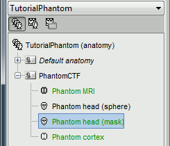
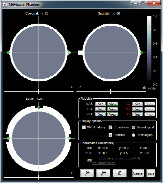
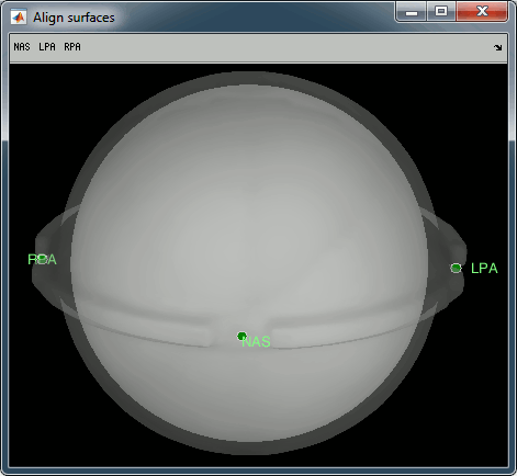
This creates a new subject PhantomCTF and generates the "anatomy" for this device: one volume and a few surfaces representing the geometry of the phantom.

You can display the MRI and surfaces as presented in the introduction tutorials.


Access the recordings
- Switch to the "functional data" view.
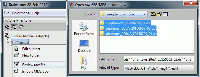
Right-click on the subject folder > Review raw file.
Select the file format: "MEG/EEG: CTF (*.ds)"
Select all the folders in: sample_phantom_ctf/ds.

- Each folder corresponds to one dataset:
emptyroom_20150709_01.ds: Phantom inside the MEG helmet, but not plugged in
phantom_20uA_20150603_03.ds: Phantom active, 23Hz, 20uA, [0,-1.8,4.9]cm
phantom_200uA_20150709_01.ds: Phantom active, 7Hz, 200uA, [0,-1.8,4.9]cm
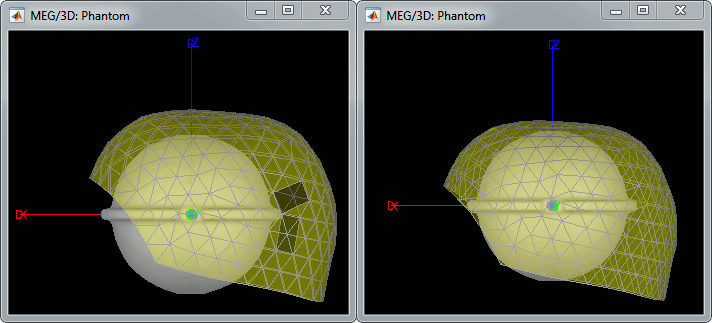
The recordings were acquired on different days, the position of the phantom in the MEG helmet is not the same for the two runs. Left = 20uA, Right = 200uA

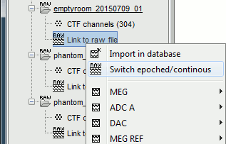
For each of the three runs: right-click on "Link to raw file" > Switch epoched/continuous

Import recordings
Event detection
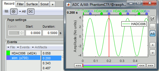
The sinusoidal signal is generated by the CTF hardware on channel HDAC006. While there are some automatic trigger events generated by the system that can be used for importing, we will have a more precise event average if the events are detected again offline.
- In Process1: Select the 20uA and 200uA links, then click on [Run].
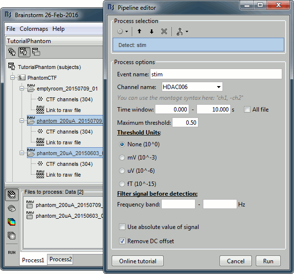
Select process: Events > Detect events above threshold
Event name=stim, Channel name=HDAC006, Time window=[0,10]s, Max thresh=0.5, Units=None, No filter, Uncheck absolute value, Check remove DC.

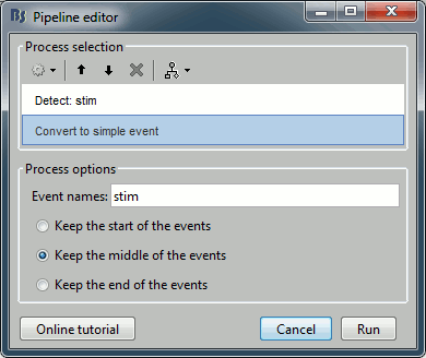
Add the process Events > Convert to simple event:
Event names=stim, Keep the middle of the events.


Import and average
- In Process1: Keep the same files selected (20uA and 200uA links), then click on [Run].
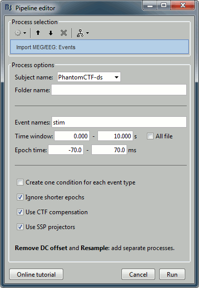
Select process: Import > Import recordings > Import MEG/EEG: Events:
Subject name=PhantomCtf, Event names=stim, Time window=[0,10]s, Epoch time=[-70,70]ms,
Uncheck Create one condition, Check the last three boxes.
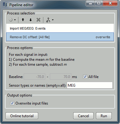
Add process Pre-process > Remove DC offset: All file, Sensor types=MEG, check Overwrite.
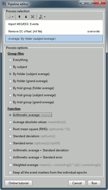
Add process Average > Average files: By folder (subject average). Run the pipeline.


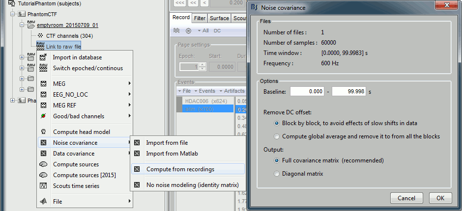
Noise covariance
Use the empty room recordings.
Right-click on the empty room Link to raw file > Noise covariance > Compute from recordings: Baseline=[0,998.3]ms, select Block by block, Full matrix.

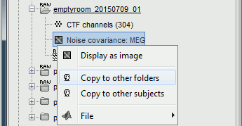
Right-click on the Noise covariance: MEG > Copy to other folders.

Source estimation
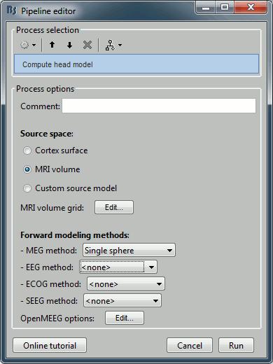
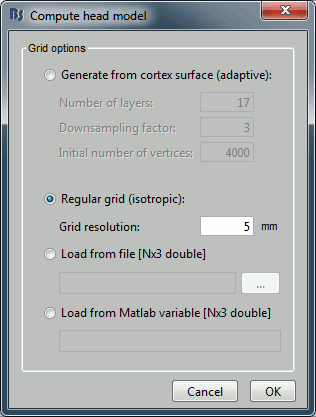
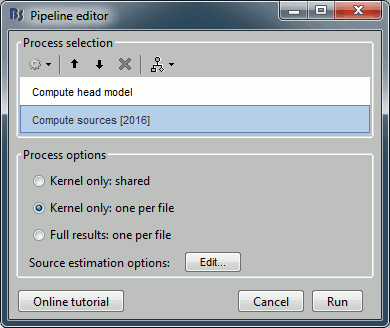
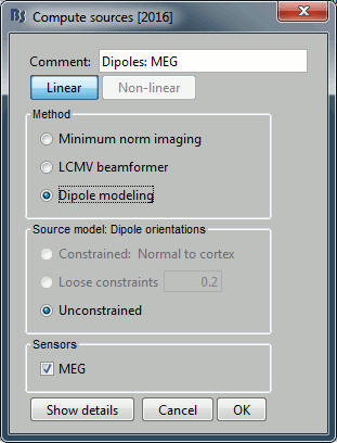
Compute a forward model and inverse model for a regular grid inside the phantom volume.
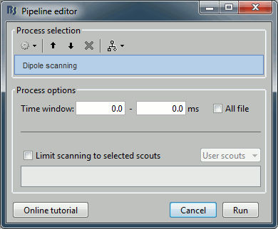
Dipole scanning
Scan the for the most significant dipole in the grid of computed dipoles estimate previously.
In Process1, select the source maps for the two conditions (20uA and 200uA)
or leave the averaged recordings selected and click on [Process sources].

Run process Sources > Dipole scanning: Time window=[0,0]ms


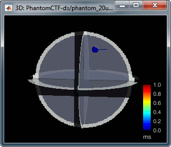
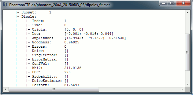
Right-click on the dipole file > File > View file contents:

Note that there is no non-linear fitting in this process. This operation selects a dipole in the grid of points available in the grid with a 5mm spacing we used during the computation of the forward model. Therefore the localisation cannot be more precise than the resolution of the grid, all the results have to interpreted with an uncertainty of +/-2.5mm.
- For a higher spatial resolution, you just need to recompute another forward model with a denser grid (2mm spacing for a 1mm precision).
Dipole fitting with FieldTrip
Perform a non-linear dipole fit with the function ft_dipolefitting from the FieldTrip toolbox.
- In Process1, select the average recordings for the two conditions (20uA and 200uA).
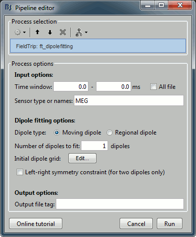
Run process Sources > FieldTrip: ft_dipolefitting: Time window=[0,0], Sensor type=MEG

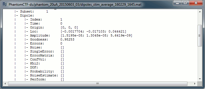
Right-click on the dipole file > File > View file contents:

- The dipoles obtained with this non-linear dipole fitting method generally have a higher goodness of fit and a more accurate location than the dipole scanning previously illustrated. But this precision comes with computation costs that can be significantly higher in the case of more realistic head models.
More information about this process in the Dipole fitting tutorial.
Results comparison
Condition |
Method |
Forward model |
X |
Y |
Z |
GOF |
|
Nominal location |
|
0 |
-18 |
49 |
mm |
200uA |
Scanning (5mm) |
Single sphere |
-1.00 |
-16.00 |
44.00 |
99.80% |
|
Scanning (5mm) |
Overlapping spheres |
-1.00 |
-16.00 |
44.00 |
99.81% |
|
Scanning (5mm) |
OpenMEEG BEM |
-1.00 |
-16.00 |
44.00 |
99.76% |
|
Fitting |
Single sphere |
-1.04 |
-17.00 |
43.98 |
99.95% |
|
Fitting |
Overlapping spheres |
-1.05 |
-16.98 |
44.00 |
99.95% |
|
CTF software |
|
-1 |
-17 |
44 |
99.95% |
|
MNE software |
|
-0.79 |
-17.00 |
43.98 |
99.9% |
|
|
|
|
|
|
|
20uA |
Scanning (5mm) |
Single sphere |
-1.00 |
-16.00 |
44.00 |
96.94% |
|
Scanning (5mm) |
Overlapping spheres |
-1.00 |
-16.00 |
44.00 |
96.96% |
|
Scanning (5mm) |
OpenMEEG BEM |
-1.00 |
-16.00 |
44.00 |
96.90% |
|
Fitting |
Single sphere |
-1.75 |
-17.13 |
44.39 |
98.25% |
|
Fitting |
Overlapping spheres |
-1.78 |
-17.14 |
44.45 |
98.25% |
|
CTF software |
|
-1 |
-17 |
44 |
98.38% |
|
MNE software |
|
-1.38 |
-16.31 |
44.01 |
99.1% |
The nominal location indicates where the dipole is supposed to be, relative to the center of the sphere. It is measured with rulers with an overall precision of about 5mm. The range of discrepancy we observe between this nominal location and the position of the dipole estimated from the recordings is acceptable.
Advanced
Digitized head points
The head points collected with the Brainstorm digitizer are usually copied to the .ds folders and imported automatically when loading the recordings. We decided not to include them in this example because in the case of this current phantom, there is no ambiguity in the definition of the anatomical fiducials. As this refined registration with the .pos files is not part of the standard CTF workflow, not including it will make it easier to compare the workflow and results with other programs.
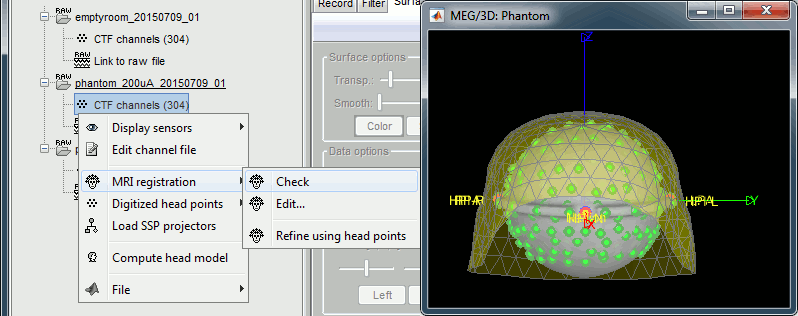
For additional testing purposes, the .pos file for the phantom is included in the sample_phantom_ctf.zip package, but you have to add it manually to the recordings. Do not use these points to refine automatically the registration: the fitting algorithm may fail finding the best rotation around the Z axis because the phantom is completely spherical, and the registration is already close to perfection.
Right-click on one of the channel files (20uA or 200uA) > Digitized head points > Add points.
Select the file format: "EEG: Polhemus"
Select file: sample_phantom_ctf/ds/phantom_20160222_01.pos

Right-click on the channel file > MRI registration > Check.

Scripting
A script available in the Brainstorm distribution reproduces the different steps of this tutorial:
brainstorm3/toolbox/script/tutorial_phantom_ctf.m
1 function tutorial_phantom_ctf(tutorial_dir)
2 % TUTORIAL_PHANTOM_CTF: Script that runs the tests for the CTF current phantom.
3 %
4 % CORRESPONDING ONLINE TUTORIAL:
5 % https://neuroimage.usc.edu/brainstorm/Tutorials/PhantomCtf
6 %
7 % INPUTS:
8 % tutorial_dir: Directory where the sample_phantom.zip file has been unzipped
9
10 % @=============================================================================
11 % This function is part of the Brainstorm software:
12 % https://neuroimage.usc.edu/brainstorm
13 %
14 % Copyright (c) University of Southern California & McGill University
15 % This software is distributed under the terms of the GNU General Public License
16 % as published by the Free Software Foundation. Further details on the GPLv3
17 % license can be found at http://www.gnu.org/copyleft/gpl.html.
18 %
19 % FOR RESEARCH PURPOSES ONLY. THE SOFTWARE IS PROVIDED "AS IS," AND THE
20 % UNIVERSITY OF SOUTHERN CALIFORNIA AND ITS COLLABORATORS DO NOT MAKE ANY
21 % WARRANTY, EXPRESS OR IMPLIED, INCLUDING BUT NOT LIMITED TO WARRANTIES OF
22 % MERCHANTABILITY AND FITNESS FOR A PARTICULAR PURPOSE, NOR DO THEY ASSUME ANY
23 % LIABILITY OR RESPONSIBILITY FOR THE USE OF THIS SOFTWARE.
24 %
25 % For more information type "brainstorm license" at command prompt.
26 % =============================================================================@
27 %
28 % Author: Francois Tadel, 2016
29
30
31 % ===== FILES TO IMPORT =====
32 % You have to specify the folder in which the tutorial dataset is unzipped
33 if (nargin == 0) || isempty(tutorial_dir) || ~file_exist(tutorial_dir)
34 error('The first argument must be the full path to the dataset folder.');
35 end
36 % Build the path of the files to import
37 Run200FileDs = fullfile(tutorial_dir, 'sample_phantom_ctf', 'ds', 'phantom_200uA_20150709_01.ds');
38 Run20FileDs = fullfile(tutorial_dir, 'sample_phantom_ctf', 'ds', 'phantom_20uA_20150603_03.ds');
39 NoiseFileDs = fullfile(tutorial_dir, 'sample_phantom_ctf', 'ds', 'emptyroom_20150709_01.ds');
40 Run200FileFif = fullfile(tutorial_dir, 'sample_phantom_ctf', 'fif', 'phantom_200uA_20150709_01.fif');
41 Run20FileFif = fullfile(tutorial_dir, 'sample_phantom_ctf', 'fif', 'phantom_20uA_20150603_03.fif');
42 PosFile = fullfile(tutorial_dir, 'sample_phantom_ctf', 'ds', 'phantom_20160222_01.pos');
43 % Check if the folder contains the required files
44 if ~file_exist(Run200FileDs)
45 error(['The folder ' tutorial_dir ' does not contain the folder from the file sample_phantom_ctf.zip.']);
46 end
47
48 % ===== CREATE PROTOCOL =====
49 % The protocol name has to be a valid folder name (no spaces, no weird characters...)
50 ProtocolName = 'TutorialPhantom';
51 % Start brainstorm without the GUI
52 if ~brainstorm('status')
53 brainstorm nogui
54 end
55 % Delete existing protocol
56 gui_brainstorm('DeleteProtocol', ProtocolName);
57 % Create new protocol
58 gui_brainstorm('CreateProtocol', ProtocolName, 0, 0);
59 % Start a new report
60 bst_report('Start');
61
62
63 % ===== ANATOMY =====
64 % Subject name
65 SubjectNameDs = 'PhantomCTF-ds';
66 SubjectNameFif = 'PhantomCTF-fif';
67 % Generate the phantom anatomy
68 generate_phantom_ctf(SubjectNameDs);
69 generate_phantom_ctf(SubjectNameFif);
70
71 % ===== LINK CONTINUOUS FILES =====
72 % Process: Create link to raw files
73 sFilesRun200Ds = bst_process('CallProcess', 'process_import_data_raw', [], [], ...
74 'subjectname', SubjectNameDs, ...
75 'datafile', {Run200FileDs, 'CTF'}, ...
76 'channelalign', 0);
77 sFilesRun20Ds = bst_process('CallProcess', 'process_import_data_raw', [], [], ...
78 'subjectname', SubjectNameDs, ...
79 'datafile', {Run20FileDs, 'CTF'}, ...
80 'channelalign', 0);
81 sFilesNoiseDs = bst_process('CallProcess', 'process_import_data_raw', [], [], ...
82 'subjectname', SubjectNameDs, ...
83 'datafile', {NoiseFileDs, 'CTF'}, ...
84 'channelalign', 0);
85 sFilesRun200Fif = bst_process('CallProcess', 'process_import_data_raw', [], [], ...
86 'subjectname', SubjectNameFif, ...
87 'datafile', {Run200FileFif, 'FIF'}, ...
88 'channelalign', 0);
89 sFilesRun20Fif = bst_process('CallProcess', 'process_import_data_raw', [], [], ...
90 'subjectname', SubjectNameFif, ...
91 'datafile', {Run20FileFif, 'FIF'}, ...
92 'channelalign', 0);
93 sFilesRawDs = [sFilesRun200Ds, sFilesRun20Ds];
94 sFilesRawFif = [sFilesRun200Fif, sFilesRun20Fif];
95 sFilesRawAll = [sFilesRawDs, sFilesRawFif];
96
97 % Process: Convert to continuous (CTF): Continuous
98 bst_process('CallProcess', 'process_ctf_convert', [sFilesRawDs, sFilesNoiseDs], [], ...
99 'rectype', 2); % Continuous
100
101
102 % ===== ADD HEAD POINTS =====
103 % Process: Add head points
104 bst_process('CallProcess', 'process_headpoints_add', sFilesRawAll, [], ...
105 'channelfile', {PosFile, 'ASCII_NXYZ'});
106
107 % Process: Snapshot: Sensors/MRI registration
108 bst_process('CallProcess', 'process_snapshot', [sFilesRun200Ds, sFilesRun20Ds], [], ...
109 'target', 1, ... % Sensors/MRI registration
110 'modality', 1, ... % MEG (All)
111 'orient', 1, ... % left
112 'Comment', 'MEG/MRI Registration');
113
114
115 % ===== DETECT EVENTS =====
116 % Process: Detect: stim
117 bst_process('CallProcess', 'process_evt_detect_threshold', sFilesRawAll, [], ...
118 'eventname', 'stim', ...
119 'channelname', 'HDAC006', ...
120 'timewindow', [0, 99.99833333], ...
121 'thresholdMAX', 0.5, ...
122 'units', 1, ... % None (10^0)
123 'bandpass', [], ...
124 'isAbsolute', 0, ...
125 'isDCremove', 1);
126 % Process: Convert to simple event
127 bst_process('CallProcess', 'process_evt_simple', sFilesRawAll, [], ...
128 'eventname', 'stim', ...
129 'method', 2); % Keep the middle of the events
130
131
132 % ===== IMPORT EVENTS =====
133 % Process: Import MEG/EEG: Events
134 sFilesEpochsAll = bst_process('CallProcess', 'process_import_data_event', sFilesRawAll, [], ...
135 'subjectname', [], ...
136 'condition', [], ...
137 'eventname', 'stim', ...
138 'timewindow', [0, 10], ...
139 'epochtime', [-0.07, 0.07], ...
140 'createcond', 0, ...
141 'ignoreshort', 1, ...
142 'usectfcomp', 1, ...
143 'usessp', 1, ...
144 'freq', [], ...
145 'baseline', [-0.07, 0.07]); % Remove DC: Entire file
146 % Process: Average: By folder (subject average)
147 sAvgAll = bst_process('CallProcess', 'process_average', sFilesEpochsAll, [], ...
148 'avgtype', 3, ... % By folder (subject average)
149 'avg_func', 1, ... % Arithmetic average: mean(x)
150 'weighted', 0, ...
151 'keepevents', 0);
152
153 % Process: Snapshot: Recordings time series
154 bst_process('CallProcess', 'process_snapshot', sAvgAll, [], ...
155 'target', 5, ... % Recordings time series
156 'modality', 1); % MEG (All)
157 % Process: Snapshot: Recordings topography (one time)
158 bst_process('CallProcess', 'process_snapshot', sAvgAll, [], ...
159 'target', 6, ... % Recordings topography (one time)
160 'modality', 1, ... % MEG (All)
161 'time', 0);
162
163
164 % ===== NOISE COVARIANCE =====
165 % Process: Compute noise covariance
166 bst_process('CallProcess', 'process_noisecov', sFilesNoiseDs, [], ...
167 'baseline', [], ...
168 'sensortypes', 'MEG, EEG, SEEG, ECOG', ...
169 'target', 1, ... % Noise covariance
170 'dcoffset', 1, ... % Block by block, to avoid effects of slow shifts in data
171 'identity', 0, ...
172 'copycond', 1, ...
173 'copysubj', 1, ...
174 'replacefile', 1); % Replace
175 % Process: Snapshot: Noise covariance
176 bst_process('CallProcess', 'process_snapshot', sFilesNoiseDs, [], ...
177 'target', 3, ... % Noise covariance
178 'Comment', 'Noise covariance');
179
180
181 % ===== SOURCE ESTIMATION =====
182 % Define source grid options
183 VolumeGrid = struct(...
184 'Method', 'isotropic', ...
185 'nLayers', 17, ...
186 'Reduction', 3, ...
187 'nVerticesInit', 4000, ...
188 'Resolution', 0.005);
189 % Process: Compute head model
190 bst_process('CallProcess', 'process_headmodel', sAvgAll, [], ...
191 'Comment', '', ...
192 'sourcespace', 2, ... % MRI volume
193 'volumegrid', VolumeGrid, ...
194 'meg', 2); % Single sphere
195 % Define inverse options
196 InverseOptions = struct(...
197 'Comment', 'Dipoles: Single sphere', ...
198 'InverseMethod', 'gls', ...
199 'InverseMeasure', 'performance', ...
200 'SourceOrient', {{'free'}}, ...
201 'Loose', 0.2, ...
202 'UseDepth', 1, ...
203 'WeightExp', 0.5, ...
204 'WeightLimit', 10, ...
205 'NoiseMethod', 'reg', ...
206 'NoiseReg', 0.1, ...
207 'SnrMethod', 'fixed', ...
208 'SnrRms', 0.001, ...
209 'SnrFixed', 3, ...
210 'ComputeKernel', 1, ...
211 'DataTypes', {{'MEG'}});
212 % Process: Compute sources [2018]
213 sAvgSrcAll = bst_process('CallProcess', 'process_inverse_2018', sAvgAll, [], ...
214 'output', 2, ... % Kernel only: one per file
215 'inverse', InverseOptions);
216 % Process: Snapshot: Sources (one time)
217 bst_process('CallProcess', 'process_snapshot', sAvgSrcAll, [], ...
218 'target', 8, ... % Sources (one time)
219 'orient', 6, ... % back
220 'time', 0, ...
221 'threshold', 40);
222
223
224 % ===== DIPOLE SCANNING =====
225 % Process: Dipole scanning
226 sDipScan = bst_process('CallProcess', 'process_dipole_scanning', sAvgSrcAll, [], ...
227 'timewindow', [0, 0], ...
228 'scouts', {});
229 % Process: Snapshot: Dipoles
230 bst_process('CallProcess', 'process_snapshot', sDipScan, [], ...
231 'target', 13, ... % Dipoles
232 'orient', 3); % top
233
234
235 % ===== FIELDTRIP DIPOLE FITTING =====
236 % Process: FieldTrip: ft_dipolefitting
237 sDipFit = bst_process('CallProcess', 'process_ft_dipolefitting', sAvgAll, [], ...
238 'filetag', 'Single sphere', ...
239 'timewindow', [0, 0], ...
240 'sensortypes', 'MEG', ...
241 'dipolemodel', 1, ... % Moving dipole
242 'numdipoles', 1, ...
243 'symmetry', 0);
244 % Process: Snapshot: Dipoles
245 bst_process('CallProcess', 'process_snapshot', sDipFit, [], ...
246 'target', 13, ... % Dipoles
247 'orient', 3); % top
248
249
250 % ===== REPORT RESULTS: SINGLE SPHERE =====
251 strResults = ['CTF current phantom' 10 '==============================================' 10];
252 % Dipole scanning
253 strResults = [strResults, 'Single sphere / Scanning:' 10];
254 for i = 1:length(sDipScan)
255 dipMat = load(file_fullpath(sDipScan(i).FileName));
256 strResults = [strResults, sprintf(' - %s: [%1.2f, %1.2f, %1.2f]mm %1.2f%% gof\n', bst_fileparts(sDipScan(i).FileName), dipMat.Dipole(1).Loc.*1000, dipMat.Dipole(1).Goodness.*100)];
257 end
258 % Dipole fitting
259 strResults = [strResults, 'Single sphere / Fitting:' 10];
260 for i = 1:length(sDipFit)
261 dipMat = load(file_fullpath(sDipFit(i).FileName));
262 strResults = [strResults, sprintf(' - %s: [%1.2f, %1.2f, %1.2f]mm %1.2f%% gof\n', bst_fileparts(sDipFit(i).FileName), dipMat.Dipole(1).Loc.*1000, dipMat.Dipole(1).Goodness.*100)];
263 end
264 % Report results
265 bst_report('Info', 'process_dipole_scanning', [], strResults);
266 disp([10 '==============================================' 10 strResults]);
267
268
269 % ===== OVERLAPPING SPHERES =====
270 % Process: Compute head model
271 bst_process('CallProcess', 'process_headmodel', sAvgAll, [], ...
272 'Comment', '', ...
273 'sourcespace', 2, ... % MRI volume
274 'volumegrid', VolumeGrid, ...
275 'meg', 3); % Overlapping spheres
276 % Process: Compute sources [2018]
277 InverseOptions.Comment = 'Dipoles: Overlapping spheres';
278 sSrcOs = bst_process('CallProcess', 'process_inverse_2018', sAvgAll, [], ...
279 'output', 2, ... % Kernel only: one per file
280 'inverse', InverseOptions);
281 % Process: Snapshot: Sources (one time)
282 bst_process('CallProcess', 'process_snapshot', sSrcOs, [], ...
283 'target', 8, ... % Sources (one time)
284 'orient', 6, ... % back
285 'time', 0, ...
286 'threshold', 40);
287
288 % Process: Dipole scanning
289 sDipScanOs = bst_process('CallProcess', 'process_dipole_scanning', sSrcOs, [], ...
290 'timewindow', [0, 0], ...
291 'scouts', {});
292 % Process: FieldTrip: ft_dipolefitting
293 sDipFitOs = bst_process('CallProcess', 'process_ft_dipolefitting', sAvgAll, [], ...
294 'filetag', 'Overlapping spheres', ...
295 'timewindow', [0, 0], ...
296 'sensortypes', 'MEG', ...
297 'dipolemodel', 1, ... % Moving dipole
298 'numdipoles', 1, ...
299 'symmetry', 0);
300
301
302 % ===== OVERLAPPING SPHERES: REPORT RESULTS =====
303 strResults = '';
304 % Dipole scanning
305 strResults = [strResults, 'Overlapping spheres / Scanning:' 10];
306 for i = 1:length(sDipScanOs)
307 dipMat = load(file_fullpath(sDipScanOs(i).FileName));
308 strResults = [strResults, sprintf(' - %s: [%1.2f, %1.2f, %1.2f]mm %1.2f%% gof\n', bst_fileparts(sDipScanOs(i).FileName), dipMat.Dipole(1).Loc.*1000, dipMat.Dipole(1).Goodness.*100)];
309 end
310 % Dipole fitting
311 strResults = [strResults, 'Overlapping spheres / Fitting:' 10];
312 for i = 1:length(sDipFitOs)
313 dipMat = load(file_fullpath(sDipFitOs(i).FileName));
314 strResults = [strResults, sprintf(' - %s: [%1.2f, %1.2f, %1.2f]mm %1.2f%% gof\n', bst_fileparts(sDipFitOs(i).FileName), dipMat.Dipole(1).Loc.*1000, dipMat.Dipole(1).Goodness.*100)];
315 end
316 % Report results
317 bst_report('Info', 'process_dipole_scanning', [], strResults);
318 disp(strResults);
319
320
321 % ===== OPENMEEG BEM =====
322 % Process: Generate BEM surfaces (DS)
323 bst_process('CallProcess', 'process_generate_bem', [], [], ...
324 'subjectname', SubjectNameDs, ...
325 'nscalp', 362, ...
326 'nouter', 162, ...
327 'ninner', 162, ...
328 'thickness', 4, ...
329 'method', 'brainstorm');
330 % Process: Generate BEM surfaces (FIF)
331 bst_process('CallProcess', 'process_generate_bem', [], [], ...
332 'subjectname', SubjectNameFif, ...
333 'nscalp', 362, ...
334 'nouter', 162, ...
335 'ninner', 162, ...
336 'thickness', 4, ...
337 'method', 'brainstorm');
338
339 % Process: Compute head model
340 bst_process('CallProcess', 'process_headmodel', sAvgAll, [], ...
341 'Comment', '', ...
342 'sourcespace', 2, ... % MRI volume
343 'volumegrid', VolumeGrid, ...
344 'meg', 4); % OpenMEEG BEM
345 % Process: Compute sources [2018]
346 InverseOptions.Comment = 'Dipoles: OpenMEEG BEM';
347 sSrcBem = bst_process('CallProcess', 'process_inverse_2018', sAvgAll, [], ...
348 'output', 2, ... % Kernel only: one per file
349 'inverse', InverseOptions);
350 % Process: Snapshot: Sources (one time)
351 bst_process('CallProcess', 'process_snapshot', sSrcBem, [], ...
352 'target', 8, ... % Sources (one time)
353 'orient', 6, ... % back
354 'time', 0, ...
355 'threshold', 40);
356 % Process: Dipole scanning
357 sDipScanBem = bst_process('CallProcess', 'process_dipole_scanning', sSrcBem, [], ...
358 'timewindow', [0, 0], ...
359 'scouts', {});
360
361
362 % ===== OPENMEEG BEM: REPORT RESULTS =====
363 strResults = '';
364 % Dipole scanning
365 strResults = [strResults, 'OpenMEEG BEM / Scanning:' 10];
366 for i = 1:length(sDipScanBem)
367 dipMat = load(file_fullpath(sDipScanBem(i).FileName));
368 strResults = [strResults, sprintf(' - %s: [%1.2f, %1.2f, %1.2f]mm %1.2f%% gof\n', bst_fileparts(sDipScanBem(i).FileName), dipMat.Dipole(1).Loc.*1000, dipMat.Dipole(1).Goodness.*100)];
369 end
370 % Report results
371 bst_report('Info', 'process_dipole_scanning', [], strResults);
372 disp(strResults);
373
374
375
376 % Save and display report
377 ReportFile = bst_report('Save', []);
378 bst_report('Open', ReportFile);
379
380
