Simulations
Author: Francois Tadel
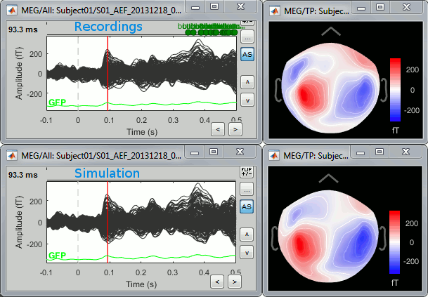
This tutorial addresses everything that can be called "simulation" in Brainstorm: simulation of simple signals, simulation of full source maps from a few scouts, simulation of MEG/EEG recordings from source maps (real or synthetic). Its goal is to group all the information that was previously spread across multiple tutorials and forum posts, and difficult to access. The examples are based on the introduction tutorials, but can easily be transposed to any study.
Contents
Simulate signals
You have no data in your database. The processes in the Simulate menu can generate signals and save them as new files in the database. Because you start from nothing, the Process1 list needs to be empty. Click on Run and try the following processes.
Simulate generic signals
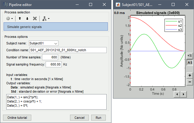
This process allows to define a set of signals with Matlab code and save it in a Brainstorm file. With the text box, you can write a free-form piece of code, which will be evaluated with the function eval(). This code must at least define the variable Data [Nsignals x Ntime], based on in the input time vector t (defined automatically by the process from the number of time points and the sampling frequency). The more rows you add to the Data matrix, the more signals you will have in your file. The example below creates three signals. Another example is available in the tutorial Time-frequency.
Simulate AR signals [TODO]
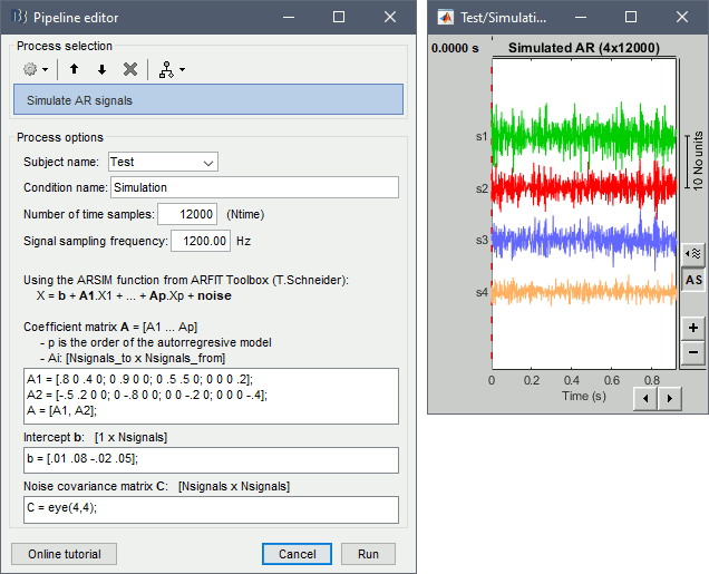
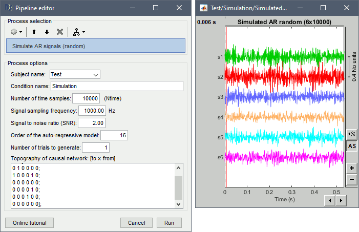
For evaluating connectivity metrics, it is useful to create signals that have known connectivity properties. Simulating signals with auto-regressive models is a solution illustrated in the tutorial Connectivity. Two processes are available, using different methods.
Process > Simulate AR signals (ARfit)
Process > Simulate AR signals (random)
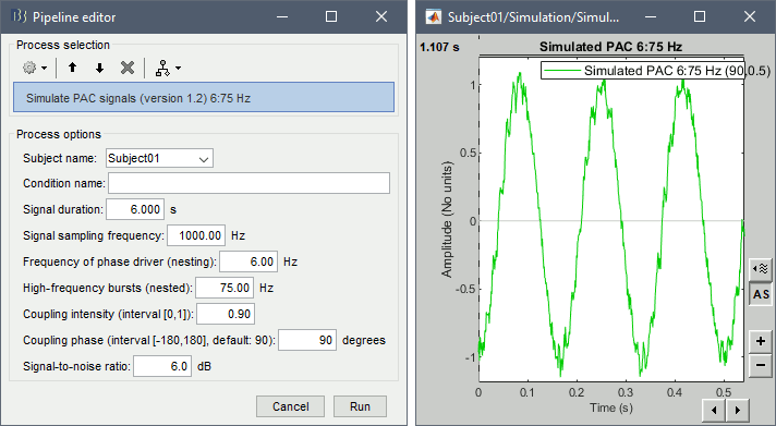
Simulate PAC signals
This process generates synthesized data containing cross-frequency phase-amplitude coupling. It is fully documented in the tutorial Phase-amplitude coupling: Method.
Simulate MEG/EEG from sources
After estimating the sources from real MEG/EEG recordings with the minimum norm method, you can simulate recordings from the model. This is done by multiplying the source time series with the forward model:
EEG_sim [Nelec x Ntime] = Forward_model [Nelec x Nsources] * MN_sources [Nsources x Ntime]
From full source maps
To simulate MEG/EEG recordings from a minimum norm source model: right-click on the source file, then select the menu Model evaluation > Simulate recordings. This can be useful for evaluating the quality of the model. The process is documented in the tutorial Source estimation.

From scouts
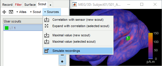
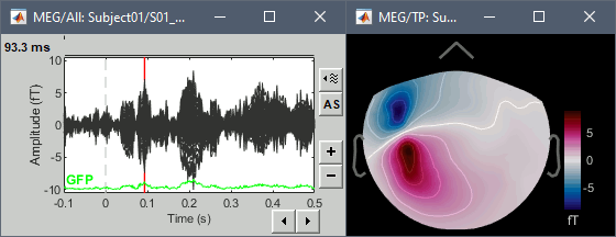
If you want to limit this simulation to a specific ROI, one easy solution is to set all the sources outside of the ROI to zero, and calculate the MEG/EEG signal exactly as above. This creates a new file which represents the scalp MEG/EEG recordings if only the selected region of the cortex was activated. Double-click on the source file to open it for display, then in the Scout tab select the scout(s) of interested and use the menu Sources > Simulate recordings.
Generate full source maps from scouts
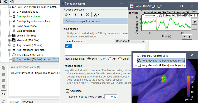
You have the values corresponding to the activity of one or a few dipoles, and you would like to save this a source file in the Brainstorm database. This source file can later be used to simulate MEG/EEG recordings, or be exported as a .nii volume or .gii surface.
Select the scouts time series in the Process1 tab, then run the process Simulate > Full source maps from scouts. Then select the scouts corresponding to the signals in input. Each input file is processed independently and results in the creation of one source file. You need a channel file and a head model file available in the same folder as the input files.
For constrained dipole orientations, you need one signal in the input file for each selected scout.
For unconstrained dipole orientations, you need three signals for each selected scout.
The order of the signals must match the order of the scouts. In the unconstrained case, the signals must be sorted by scout and then by orientation (scout1_orientX, scout1_orientY, scout1_orientZ, scout2_orientX...). In the process options, you cannot change the order of the scouts, however you can re-arrange them if you generate a script.
This process is the first step executed by the process "Simulate > Simulate recordings from scouts", illustrated in the following section.
Simulate MEG/EEG from synthetic dipoles
You have the values corresponding to the activity of one or a few dipoles, and you would like to simulate the corresponding MEG/EEG surface recordings. The process Simulate > Simulate recordings from scouts does this as a combination of two mechanisms previously described on this page: 1) it generates a source map with zeros everywhere except for a few scouts where it uses instead the signals provided in the input file (see previous section), 2) it multiplies this source map with the forward model available in the folder to simulate MEG/EEG recordings. Noise can be added at each stage.
The input signals can be simulated (as explained in the first sections of this page) or extracted from sources estimated from real MEG/EEG recordings (also explained earlier in this page). You need to provide one signal per scout for constrained sources, or three signals per scout for unconstrained sources. The examples below illustrate three types of source models: cortex surface / constrained orientation, cortex surface / unconstrained orientation, volume grid / unconstrainted orientation.
Surface: Constrained orientation
Simulation of a single dipole located on the cortex surface, oriented along the normal to the cortex surface, pointing outwards.
Go to functional view of the protocol TutorialIntroduction.
Right-click on Subject01 > New folder: "Simulation1".
Copy-paste the channel file, the noise covariance and the head model "Overlapping sphere" from the imported folder for the first acquisition run (S01_AEF_20131218_01_600Hz_notch): use CTRL+C/CTRL+V or the popup menus File > Copy/Paste.

- From the anatomy view of the process, double-click on the low-resolution pial surface (cortex_15002V) to display it.
Menu Atlas > New atlas > Empty atlas: "Simulation1".
Create a new scout, do not grow it, name it dip1 (detailed instructions).

- Go back to the functional view of the process.
Empty the Process1 box, click on Run, execute the process Simulate > Simulate generic signal, configured as illustrated below.
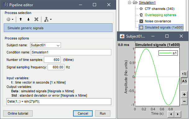
- Select the simulated signal in Process1.
Run the process Simulate > Simulate recordings from scouts, selecting the scout Simulation1/dip1.
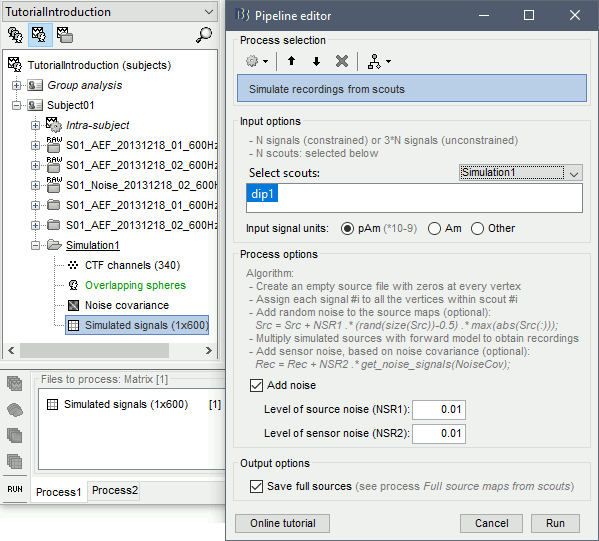
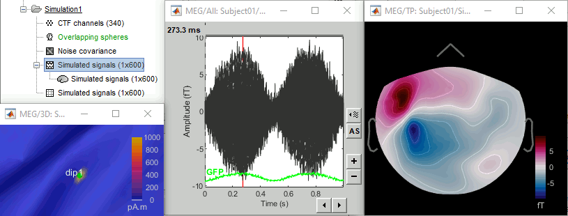
- Open the source file generated for this simulation: All the vertices are set to zero (plus some noise), except for one vertex that has been assigned the values of the simulated signal s1.
Open the simulated MEG recordings and a 2D topography. Scroll in time to observe the flip of orientation of the dipole after 500ms. This simulation was based on only one dipole, with a fixed orientation along the normal to the cortex, and pointing outwards (see tutorial Source estimation).
Units: In this simulation, we didn't pay much attention to the signal units. We used a source signal with no units and an amplitude of 1, while the amplitude of the current density maps estimated with the minimum norm method are supposed to be in the range of a few pA.m (1e-12). If the maximum value is lower than 1e-3, the function process_simulate_recordings.m multiplies the signals in input by 1e-9. It does not have any physical meaning, but it allows to obtain MEG/EEG values in a range that can be represented by Brainstorm visualization tools. If you want to obtain meaningful units for the simulated MEG/EEG data, you should use input signals that are appropriately scaled in pA.m.
- Repeat the experiment with different amounts of source noise (SNR1) and sensor noise (SNR2).
Surface: Unconstrained orientation
Simulation of three dipoles at the same location on the cortex surface, oriented along three orthogonal axes (X,Y,Z) as defined in the SCS coordinate system.
- Create a new folder: "Simulation3"
Copy-paste the channel file, the noise covariance and the head model "Overlapping sphere" from the Simulation1 folder (or the first acquisition run S01_AEF_20131218_01_600Hz_notch).

We will reuse the same scout dip1 defined in the previous simulation.
Empty the Process1 box, click on Run, execute the process Simulate > Simulate generic signal, configured as illustrated below.
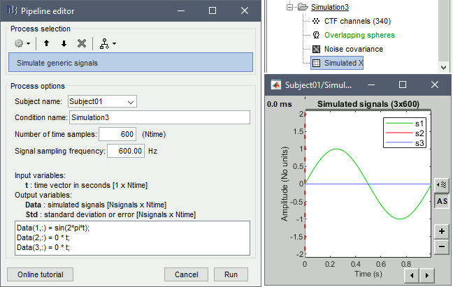
Rename the output file "Simulated X" (right-click > File > Rename, or F2).
This is the same signal as previously, but defined with 2 other empty signals (zero at all the time samples) in the same file. When matching the file with the scout dip1, the simulation process will no longer use the normal to the cortex, it will use the first signal as the dipole along the X axis, the second along the Y axis, and the third along the Z axis. Therefore it will simulate a dipole oriented along the X axis. To display the axes on a 3D figure: right-click on the figure > Figure > Show axis (or CTRL+A).
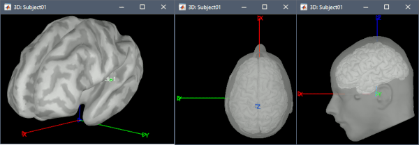
Red: X (from back to front), Green: Y (from right to left), Blue: Z (from bottom to top).- Select the simulated signals in Process1.
Run the process Simulate > Simulate recordings from scouts, selecting the scout Simulation1/dip1.
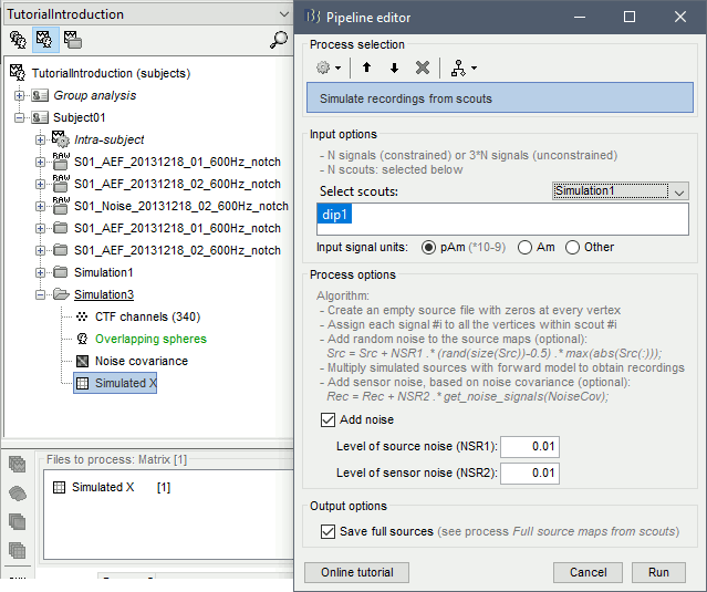
Display the simulated recordings and a 2D topography.

Repeat the procedure to generate the signals for the Y and Z axes. The main difference is the simulation of the signal: for Y, set Data(1,:)=0*t and Data2(2,:)=the sinusoid. For Z, define the sinusoid in the third signal Data(3,:).


- The patterns of the magnetic fields we obtained correspond to what we expect:
- Simulated X: dipole oriented from back to front.
- Simulated Y: dipole oriented radially with respect with the surface of the head, therefore almost invisible with MEG.
- Simulated Z: dipole oriented from right to left.
Volume: Unconstrained orientation
In the first two examples, we showed how to reuse existing recordings already imported and processed. If you don't have any real MEG/EEG recordings to start with, you may not have any channel file a noise covariance to use in your simulation.
In this third example, we will demonstrate how to simulate EEG activity using a template anatomy and a standard 10-10 electrode cap, and from a dipole in a volume grid instead of the cortex surface.
Prepare head model
Create a new subject Simulation, with the option "Default anatomy: Yes".
Create a new folder VolumeEEG within the new subject.
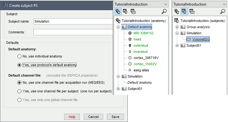
Right-click on the new folder > Use default EEG cap > ICBM152 > Generic > 10-10 65.
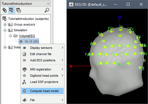
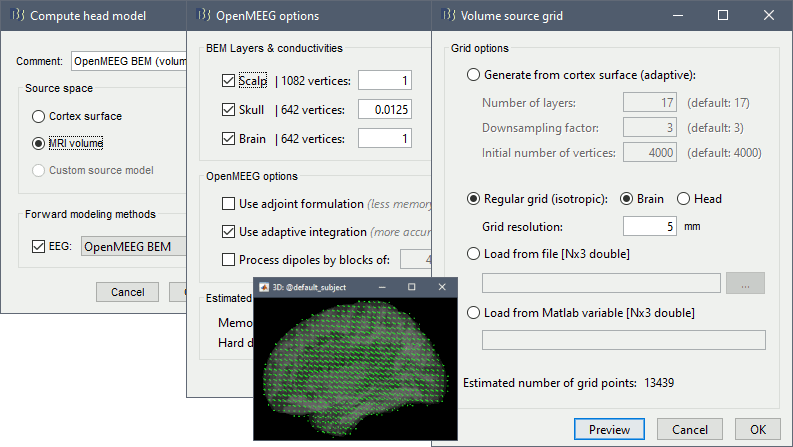
Right-click on the channel file > Compute head model, with the following options selected:
MRI volume: See tutorial Volume source estimation
OpenMEEG BEM: See tutorial Realistic head model: BEM with OpenMEEG
OpenMEEG options: Keep all the default
Volume source grid: Regular grid (isotropic) / Brain / 5mm
Create volume scout
Right-click on the head model > Check source grid (MRI)
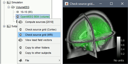
In the Scout tab, menu Atlas > New atlas > Volume scouts.
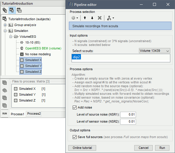
Create a new scout with one grid point onlt, close to the scout you used in the previous simulations, in order to compare the topographies between EEG and MEG. Rename it dip2. For help, see the tutorials Scouts and Volume source estimation.

Noise covariance
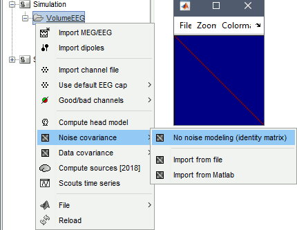
Right-click on the folder: Noise covariance > No noise modeling (identity matrix).
Simulation
We will reuse the same signals as in the previous simulation (Surface: Unconstrained orientation). You can simply copy-paste the simulated signals Simulation X/Y/Z (the "matrix" files, not the simulated MEG recordings) to the folder Simulation/VolumeEEG.
Select the three simulated signals X/Y/Z and run the process Simulate > Simulate recordings from scouts, selecting the scout Volume/dip2.
Display the simulated EEG time series and topographies for the three dipole orientations.


If you want to double-check that you simulated correctly your dipoles: double-click to open the source file for Simulated X. In the scout tab, select the dip2 dipole and the option Values:Relative, then click on the button Display scouts time series. You should get the 3 signals you designed, plus some additional noise.

Additional documentation
Articles
A simulation article was published by Prof. Debener's neuropsychology lab in Oldenburg. It uses Brainstorm to evaluate and improve the design of ear-EEG devices. All the Matlab/Brainstorm scripts used in this study are available on figshare, together with some videos illustrating the simulations that were done.
Meiser A, Tadel F, Debener S, Bleichner MG
The Sensitivity of Ear-EEG: Evaluating the Source-Sensor Relationship Using Forward Modeling
Brain Topography, Aug 2020

Forum discussions
Simulate recordings from sources: http://neuroimage.usc.edu/forums/showthread.php?2563
Simulate recordings from simulated signals: https://neuroimage.usc.edu/forums/t/simulate-scalp-recording/2421/3
Scripting
The following script from the Brainstorm distribution reproduces the third example presented in this tutorial page (Volume: Unconstrained orientation): brainstorm3/toolbox/script/tutorial_simulations.m
