Tutorial 26: Statistics

Authors: Francois Tadel, Elizabeth Bock, Dimitrios Pantazis, Richard Leahy, Sylvain Baillet

In this auditory oddball experiment, we would like to test for the significant differences between the brain response to the deviant beeps and the standard beeps, time sample by time sample. Until now we have been computing measures of the brain activity in time or time-frequency domain. We were able to see clear effects or slight tendencies, but these observations were always dependent on an arbitrary amplitude threshold and the configuration of the colormap. With appropriate statistical tests, we can go beyond these empirical observations and assess what are the significant effects in a more formal way.

Random variables

In most cases we are interested in comparing the brain signals recorded for two populations or two experimental conditions A and B.

A and B are two random variables for which we have a limited number of repeated measures: multiple trials in the case of a single subject study, or multiple subject averages in the case of a group analysis. To start with, we will consider that each time sample and each signal (source or sensor) is independent: a random variable represents the possible measures for one sensor/source at one specific time point.

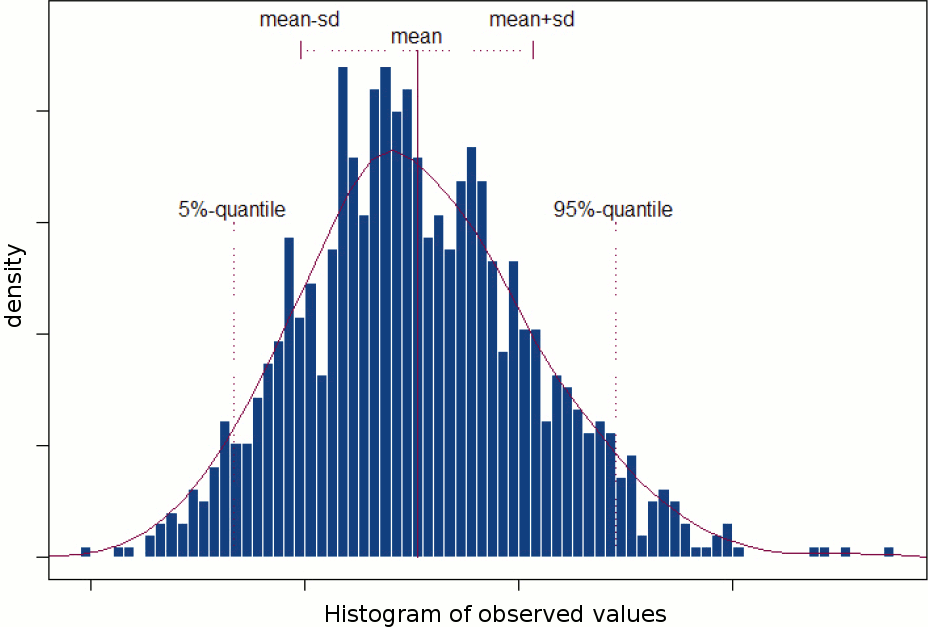
A random variable can be described with its probability distribution: a function which indicates what are the chances to obtain one specific measure if we run the experiment. By repeating the same experiment many times, we can approximate this function with a discrete histogram of observed measures.

Histograms

You can plot histograms like this one in Brainstorm, it may help you understand what you can expect from the statistics functions described in the rest of this tutorial. For instance, seeing a histogram computed with only 4 values would discourage you forever from running a group analysis with 4 subjects...

Recordings

• Let's evaluate the recordings we obtained for sensor MLP57, the channel that was showing the highest value at 160ms in the difference of averages computed in the previous tutorial.
  
  

• We are going to extract only one value for each trial we have imported in the database, and save these values in two separate files, one for each condition (standard and deviant).
  In order to observe more meaningful effects, we will process the trials together from the two acquisition runs. As explained in the previous tutorials (link), this is usually not recommended in MEG analysis, but it can be an acceptable approximation if the subject didn't move between runs.

• In Process1, select all the deviant trials from both runs.
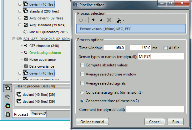
  Run process Extract > Extract values:
  Options: Time=[160,160]ms, Sensor="MLP57", Concatenate time (dimension 2)
  
  

• Repeat the same operation for all the standard trials.

• You obtain two new files in the folder Intra-subject. If you look inside the files, you can observe that the size of the Value matrix matches the number of trials (78 for deviant, 383 for standard). The matrix is [1 x Ntrials] because we asked to concatenate the extracted values in the 2nd dimension.
  
  

• To display the distribution of the values in these two files:
  select them simultaneously, right-click > File > View histograms.
  
  

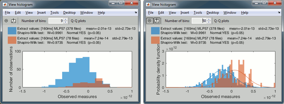
• With the buttons in the toolbar, you can edit the way these distributions are represented: number of bins in the histogram, total number of occurrences (shows taller bars for standard because it has more values) or density of probability (normalized by the total number of values).
  In addition, you can plot the normal distribution corresponding to the mean μ and standard deviation σ computed from the set of values (using Matlab functions mean and std).

• When comparing two sample sets A and B, we try to evaluate if the distributions of the measures are equal or not. In most of the questions we explore in EEG/MEG analysis, the distributions are overlapping a lot. The very sparse sampling of the data (a few tens or hundreds of repeated measures) doesn't help with the task. Some representations will be more convincing than others to estimate the differences between the two conditions.
  
  

• The legend of the histograms shows the result of the Shapiro-Wilk normality test, as implemented by Ahmed BenSaïda (Matlab FileExchange). The button "Q-Q plots" gives another way to compare the current samples to the normal distribution (see: Wikipedia, Matlab FileExchange).
  
  

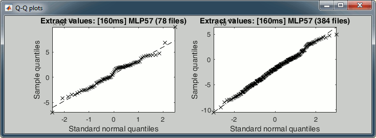
• Everything seems to indicate that the values recorded on the sensor MLP57 at 160ms follow a normal distribution, in both conditions.

Sources (relative)

• We can repeat the same operation at the source level and extract all the values for scout A1L.

• In Process1, select all the deviant trials from both runs. Select button [Process sources].
  Run process Extract > Extract values: Time=[160,160]ms, Scout="A1L"
  
  

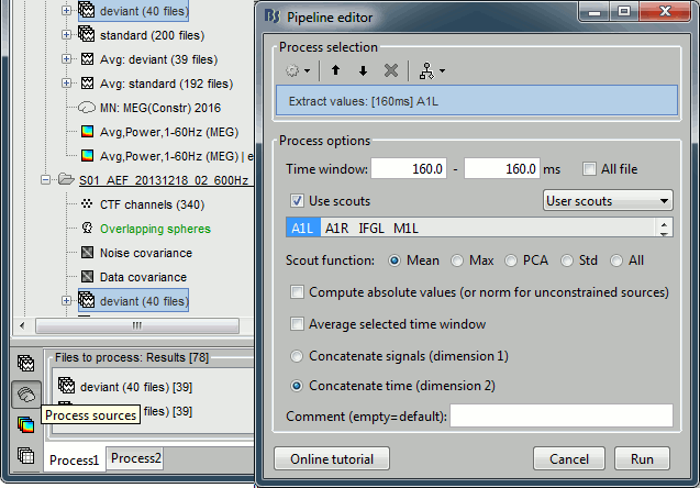
• Repeat the same operation for all the standard trials.

• Select the two files > Right-click > File > View histogram.
  
  

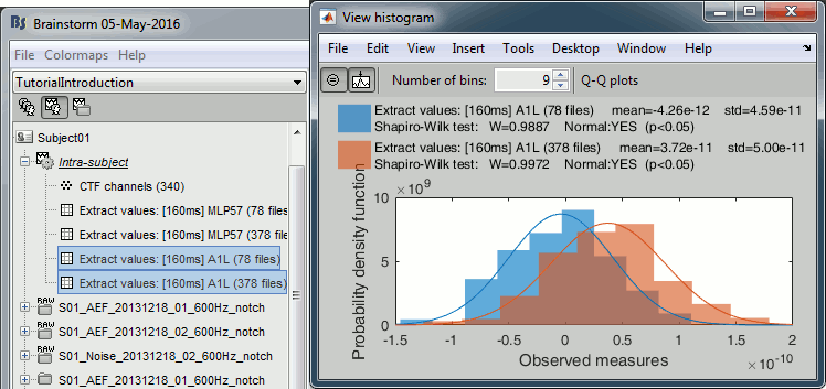
• The distributions still look normal, but the variances are now slightly different. You have to pay attention to this information when choosing which parametric t-test to run.

Sources (absolute)

• Run again the process Extract > Extract values, but this time select Compute absolute values.

• Display the histograms of the two rectified files.
  
  

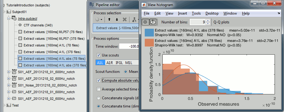
• The rectified source values are definitely not following a normal distribution, the shape of the histogram has nothing to do with the corresponding Gaussian curves. As a consequence, if you are using rectified source maps, you will not be able to run independent parametric t-tests.
  Additionally, you may have issues with the detection of some effects (see tutorial Difference).

Time-frequency

• Time-frequency power for sensor MLP57 at 55ms / 48Hz (left=no normalization, right=ERS/ERD):
  
  

• These sample sets are clearly not normally distributed. Parametric t-tests don't look like good candidates for testing time-frequency power across trials.

Group studies and central limit theorem

• The observations above hold only for the specific case we are looking at: single subject analysis, testing for differences across trials.

• In the context of a group analysis, we usually test subject averages between conditions or populations. This corresponds to comparing the distributions of the mean of the trials across subjects, which will tend to be normal when we increase the number of trials (Central-limit theorem). In general, it is easier to obtain sample sets with normal distributions at the group level.

• Additionally, some tricks can help bringing the samples closer to a normal distribution, like averaging in time/space/frequencies, or testing the square root of the data, in the case of time-frequency power. Some solutions are explored in (Kiebel, Tallon-Baudry & Friston, HBM 2005).

Statistical inference

Hypothesis testing

To show that there is a difference between A and B, we can use a statistical hypothesis test. We start by assuming that the two sets are identical then reject this hypothesis. For all the tests we will use here, the logic is similar:

• Define a null hypothesis (H₀:"A=B") and an alternative hypothesis (eg. H₁:"A<B").

• Make some assumptions on the samples we have (eg. A and B are independent, A and B follow normal distributions, A and B have equal variances).

• Decide which test is appropriate, and state the relevant test statistic T (eg. Student t-test).

• Compute from the measures (A_obs, B_obs) the observed value of the test statistic (t_obs).

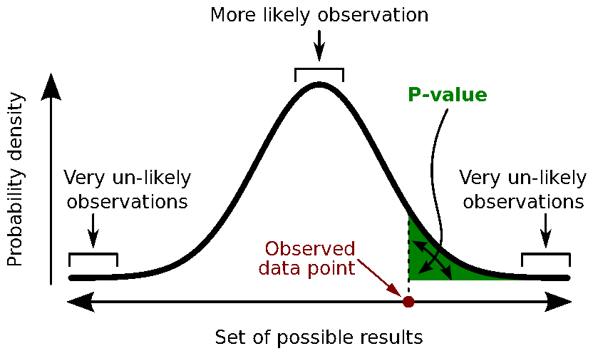
• Calculate the p-value. This is the probability, under the null hypothesis, of sampling a test statistic at least as extreme as that which was observed. A value of (p<0.05) for the null hypothesis has to be interpreted as follows: "If the null hypothesis is true, the chance that we find a test statistic as extreme or more extreme than the one observed is less than 5%".

• Reject the null hypothesis if and only if the p-value is less than the significance level threshold (α).
  
  

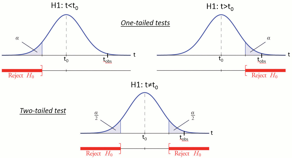
Evaluation of a test

The quality of test can be evaluated based on two criteria:

• Sensitivity: True positive rate = power = ability to correctly reject the null hypothesis and control for the false negative rate (type II error rate). A very sensitive test detects a lot of significant effects, but with a lot of false positive.

• Specificity: True negative rate = ability to correctly accept the null hypothesis and control for the false positive rate (type I error rate). A very specific test detects only the effects that are clearly non-ambiguous, but can be too conservative and miss a lot of the effects of interest.
  
  

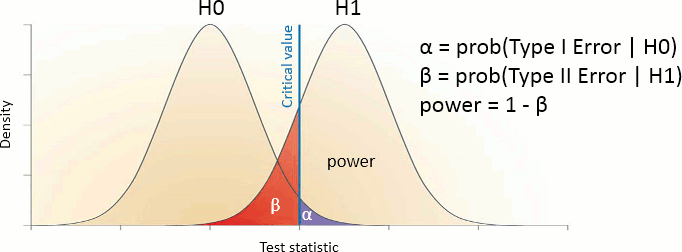
Different categories of tests

Two families of tests can be helpful in our case: parametric and nonparametric tests.

• Parametric tests need some strong assumptions on the probability distributions of A and B then use some well-known properties of these distributions to compare them, based on a few simple parameters (typically the mean and variance). The estimation of these parameters is highly optimized and requires very little memory. The examples which will be described here are the Student's t-tests.

• Nonparametric tests do not require any assumption on the distribution of the data. They are therefore more reliable and more generic. On the other hand, they are a lot more complicated to implement: they require a lot more memory because all the tested data has to be loaded at once, and a lot more computation time because the same test is repeated thousands of times.

Parametric Student's t-test

Assumptions

The Student's t-test is a widely-used parametric test to evaluate the difference between the means of two random variables (two-sample test), or between the mean of one variable and one known value (one-sample test). If the assumptions are correct, the t-statistic follows a Student's t-distribution.

• 

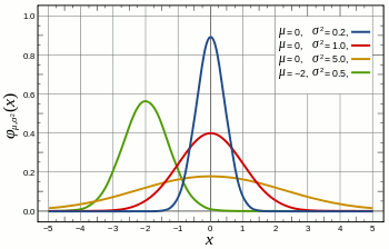
The main assumption for using a t-test is that the random variables involved follow a normal distribution (mean: μ, standard deviation: σ). The figure below shows a few example of normal distributions.

• 

t-statistic

Depending on the type of data we are testing, we can have different variants for this test:

• One-sample t-test (testing against a known mean μ₀):
  
  where is the sample mean, σ is the sample standard deviation and n is the sample size.

• Dependent t-test for paired samples (eg. when testing two conditions across a group of subjects). Equivalent to testing the difference of the pairs of samples against zero with a one-sample t-test:
  
  where D=A-B, is the average of D and σ_D its standard deviation.

• Independent two-sample test, equal variance (equal or unequal sample sizes):
  
  where and are the unbiased estimators of the variances of the two samples.

• Independent two-sample test, unequal variance (Welch's t-test):
  
  where and are the sample sizes of A and B.

p-value

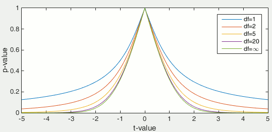
Once the t-value is computed (t_obs in the previous section), we can convert it to a p-value based on the known distributions of the t-statistic. This conversion depends on two factors: the number of degrees of freedom and the tails of the distribution we want to consider. For a two-tailed t-test, the two following commands in Matlab are equivalent and can convert the t-values in p-values.

p = betainc(df./(df + t.^2), df/2, 0.5);    % Without the Statistics toolbox
p = 2*(1 - tcdf(abs(t),df));                % With the Statistics toolbox

The distribution of this function for different numbers of degrees of freedom:

• 

Example 1: Parametric t-test on recordings

Parametric t-tests require the values tested to follow a normal distribution. The recordings evaluated in the histograms sections above (MLP57/160ms) show distributions that are matching this assumption relatively well: the histograms follow the traces of the corresponding normal functions, and the two conditions have very similar variances. It looks reasonable to use a parametric t-test in this case.

• In the Process2 tab, select the following files, from both runs (approximation discussed previously):

  • Files A: All the deviant trials, with the [Process recordings] button selected.

  • Files B: All the standard trials, with the [Process recordings] button selected.

  • The t-tests work well with unbalanced number of samples: It is better to use all the possible samples you have, even if you have 80 trials in one condition and 400 in the other.

• Run the process "Test > Parametric test: Independent": Select all the data, do not average.
  Sensor types: Leave this empty instead of entering "MEG", it won't affect the results but the computation will be faster (optimized when processing full files).
  Test: Student's t-test (equal variance), two-tailed.
  
  

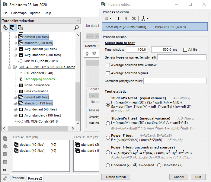
• Double-click on the new file and add a 2D topography (CTRL+T). The values displayed in the 2D view are the significant t-values. All the sensors that have p-values higher than the significance level threshold (α) are set to zero.

• With the new Stat tab you can control the significance level α and the correction you want to apply for multiple comparisons (see next section).

• With the option minimum duration, you can exclude from the display all the data points that are significant only for isolated time samples, and which are mostly likely false positives. If this parameter is set to zero it has no impact on the display. Otherwise all the data points that are not significant continuously for at least this duration are set to zero.
  
  

Correction for multiple comparisons

Multiple comparison problem

The approach described in this first example performs many tests simultaneously. We test, independently, each MEG sensor and each time sample across the trials, so we run a total of 274*361 = 98914 t-tests.

If we select a critical value of 0.05 (p<0.05), it means that we want to see what is significantly different between the conditions while accepting the risk of observing a false positive in 5% of the cases. If we run the test around 100,000 times, we can expect to observe around 5,000 false positives. We need to better control for false positives (type I errors) when dealing with multiple tests.

Bonferroni correction

The probability to observe at least one false positive, or familywise error rate (FWER) is almost 1:
FWER = 1 - prob(no significant results) = 1 - (1 - 0.05)^100000 ~ 1

A classical way to control the familywise error rate is to replace the p-value threshold with a corrected value, to enforce the expected FWER. The Bonferroni correction sets the significance cut-off at /Ntest. If we set (p ≤ /Ntest), then we have (FWER ≤ ). Following the previous example:
FWER = 1 - prob(no significant results) = 1 - (1 - 0.05/100000)^100000 ~ 0.0488 < 0.05

This works well in a context where all the tests are strictly independent. However, in the case of MEG/EEG recordings, the tests have an important level of dependence: two adjacent sensors or time samples often have similar values. In the case of highly correlated tests, the Bonferroni correction tends too be conservative, leading to a high rate of false negatives.

FDR correction

The false discovery rate (FDR) is another way of representing the rate of type I errors in null hypothesis testing when conducting multiple comparisons. It is designed to control the expected proportion of false positives, while the Bonferroni correction controls the probability to have at least one false positive. FDR-controlling procedures have greater power, at the cost of increased rates of Type I errors (Wikipedia)

In Brainstorm, we implement the Benjamini–Hochberg step-up procedure (1995):

• Sort the p-values p(k) obtained across all the multiple tests (k=1..Ntest).

• Find the largest k such as p(k) < k / Ntest * .

• Reject the null hypotheses corresponding to the first k smallest p-values.

• This is is the same procedure as Matlab's call: mafdr(p, 'BHFDR', alpha)

Note that there are different implementations of FDR. FieldTrip uses the Benjamini–Yekutieli (2001) algorithm as described in (Genovese, 2002), which usually gives less true positive results. Don't be surprised if you get empty displays when using the option "FDR" in the FieldTrip processes, while you get significant results with the Brainstorm FDR correction.

In the interface

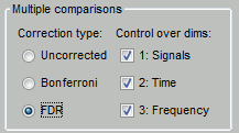
You can select interactively the type of correction to apply for multiple comparison while reviewing your statistical results. The checkboxes "Control over dims" allow you to select which are the dimensions that you consider as multiple comparisons (1=sensor, 2=time, 3=not applicable here). If you select all the dimensions, all the values available in the file are considered as the same repeated test, and only one corrected p-threshold is computed for all the time samples and all the sensors.

If you select only the first dimension, only the values recorded at the same time sample are considered as repeated tests, the different time points are corrected independently, with one different corrected p-threshold for each time point.

When changing these options, a message is displayed in the Matlab command window, showing the number of repeated tests that are considered, and the corrected p-value threshold (or the average if there are multiple corrected p-thresholds, when not all the dimensions are selected):

BST> Average corrected p-threshold: 5.0549e-07  (Bonferroni, Ntests=98914)
BST> Average corrected p-threshold: 0.00440939  (FDR, Ntests=98914)

"It doesn't work"

If nothing appears significant after correction, don't start by blaming the method ("FDR doesn't work"). In the first place, it's probably because there is no clear difference between your sample sets or simply because your sample size is too small. For instance, with less than 10 subjects you cannot expect to observe very significant effects in your data.

If you have good reasons to think your observations are meaningful but cannot increase the sample size, consider reducing the number of multiple comparisons you perform (test only the average over a short time window, a few sensors or a region of interest) or using a cluster-based approach. When using permutation tests, increasing the number of random permutations also decreases the p-value of the very significant effects.

Nonparametric permutation tests

Principle

A permutation test (or randomization test) is a type of test in which the distribution of the test statistic under the null hypothesis is obtained by calculating all possible values of the test statistic under rearrangements of the labels on the observed data points. (Wikipedia)

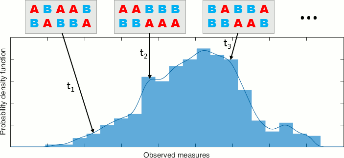
If the null hypothesis is true, the two sets of tested values A and B follow the same distribution. Therefore the values are exchangeable between the two sets: we can move one value from set A to set B, and one value from B to A, and we expect to obtain the same value for the test statistic T.

• 

By taking all the possible permutations between sets A and B and computing the statistic for each of them, we can build a histogram that approximates the permutation distribution.

• 

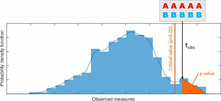
Then we compare the observed statistic with the permutation distribution. From the histogram, we calculate the proportion of permutations that resulted in a larger test statistic than the observed one. This proportion is called the p-value. If the p-value is smaller than the critical value (typically 0.05), we conclude that the data in the two experimental conditions are significantly different.

• 

The number of possible permutations between the two sets of data is usually too large to compute an exhaustive permutation test in a reasonable amount of time. The permutation distribution of the statistic of interest is approximated using a Monte-Carlo approach. A relatively small number of random selection of possible permutations can give us a reasonably good idea of the distribution.

Permutation tests can be used for any test statistic, regardless of whether or not its distribution is known. The hypothesis is about the data itself, not about a specific parameter. In the examples below, we use the t-statistic, but we could use any other function.

Practical limitations

Computation time: If you increase the number of random permutations you use for estimating the distribution, the computation time will increase linearly. You need to find a good balance between the total computation time and the accuracy of the result.

Memory (RAM): The implementations of the permutation tests available in Brainstorm require all the data to be loaded in memory before starting the evaluation of the permutation statistics. Running this function on large datasets or on source data could quickly crash your computer. For example, loading the data for the nonparametric equivalent to the parametric t-test we ran previously would require:
276(sensors) * 461(trials) * 361(time) * 8(bytes) / 1024^3(Gb) = 0.3 Gb of memory.

This is acceptable on most recent computers. But to perform the same at the source level, you need:
45000*461*361*8/1024^3 = 58 Gb of memory just to load the data. This is impossible on most computers, we have to give up at least one dimension and run the test only for one region of interest or one time sample (or average over a short time window).

Example 2: Permutation t-test

Let's run the nonparametric equivalent to the test we ran in the first example.

• In the Process2 tab, select the following files, from both runs (approximation discussed previously):

  • Files A: All the deviant trials, with the [Process recordings] button selected.

  • Files B: All the standard trials, with the [Process recordings] button selected.

• Run the process "Test > Permutation test: Independent", set the options as shown below.
  Sensor type: You should enter explicitly "MEG" instead of leaving this field empty. It will decrease the computation time (no optimization for full files in the nonparametric tests).
  Note that it may require more than 3Gb of RAM and take more than 10min.
  
  

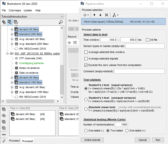
• Open the parametric and nonparametric results side by side, the results should be very similar. You may have to increase the significance level α to 0.05 to see something significant in the nonparametric version (edit the value in the Stat tab). Alternatively, you can obtain lower p-values by running the same process with more randomizations (for instance 2000 or 10000).
  
  

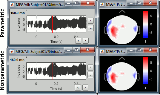
• In this case, the distributions of the values for each sensor and each time point (non-rectified MEG recordings) are very close to normal distributions. This was illustrated at the top of this page, in the section "Histograms". Therefore the assumptions behind the parametric t-test are verified, the results of the parametric tests are correct and very similar to the nonparametric ones.

• If you get different results with the parametric and nonparametric approaches: trust the nonparametric one. If you want to increase the precision of a nonparametric test a decrease the p-values, increase the number of random permutations.

MacOS troubleshooting

Error "mexmaci64 cannot be opened because the developer cannot be verified":

• Brainstorm forum

• SPM12 website

• FieldTrip website

FieldTrip implementation

FieldTrip functions in Brainstorm

We have the possibility to call some of the FieldTrip toolbox functions from the Brainstorm environment. If you are running the compiled version of Brainstorm these functions are already packaged with Brainstorm, otherwise you need to install FieldTrip on your computer, either manually or as a Brainstorm plugin. See the Plugins tutorial.

Cluster-based correction

One interesting method that has been promoted by the FieldTrip developers is the cluster-based approach for nonparametric tests. In the type of data we manipulate in MEG/EEG analysis, the neighboring channels, time points or frequency bins are expected to show similar behavior. We can group these neighbors into clusters to "accumulate the evidence". A cluster can have a multi-dimensional extent in space/time/frequency.

In the context of a nonparametric test, the test statistic computed at each permutation is the extent of the largest cluster. To reject or accept the null hypothesis, we compare the largest observed cluster with the randomization distribution of the largest clusters.

This approach solves the multiple comparisons problem, because the test statistic that is used (the maximum cluster size) is computed using all the values at the same time, along all the dimensions (time, sensors, frequency). There is only one test that is performed, so there is no multiple comparisons problem.

The result is simpler to report but also a lot less informative than FDR-corrected nonparametric tests. We have only one null hypothesis, "the two sets of data follow the same probability distribution", and the outcome of the test is to accept or reject this hypothesis. Therefore we cannot report the spatial or temporal extent of the most significant clusters. Make sure you read this recommendation before reporting cluster-based results in your publications.

Reference documentation

For a complete description of nonparametric cluster-based statistics in FieldTrip, read the following:

• Article: Maris & Oostendveld (2007)

• Video: Statistics using non-parametric randomization techniques (E Maris)

• Video: Non-parametric cluster-based statistical testing of MEG/EEG data (R Oostenveld)

• Tutorial: Parametric and non-parametric statistics on event-related fields

• Tutorial: Cluster-based permutation tests on event related fields

• Tutorial: Cluster-based permutation tests on time-frequency data

• Tutorial: How NOT to interpret results from a cluster-based permutation test

• Functions references: ft_timelockstatistics, ft_sourcestatistics, ft_freqstatistics

Process options

There are three separate processes in Brainstorm, to call the three FieldTrip functions.

• ft_timelockstatistics: Compare imported trials (recordings).

• ft_sourcestatistics: Compare source maps or time-frequency decompositions of sources.

• ft_freqstatistics: Compare time-frequency decompositions of sensor recordings or scouts signals.

• See below the correspondence between the options in the interface and the FieldTrip functions.

Test statistic options (name of the options in the interface in bold):

• cfg.numrandomization = "Number of randomizations"

• cfg.statistic = "Independent t-test" ('indepsamplesT') or "Paire t-test" ('depsamplesT)

• cfg.tail = One-tailed (-1), Two-tailed (0), One-tailed (+1)

• cfg.correctm = "Type of correction" ('no', 'cluster', 'bonferroni', 'fdr', 'max', 'holm', 'hochberg')

• cfg.method = 'montecarlo'

  
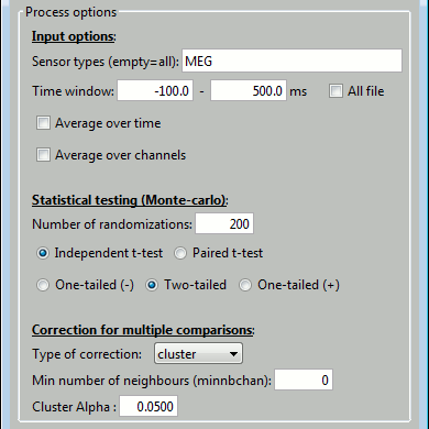
• cfg.correcttail = 'prob'

Cluster-based correction:

• cfg.clusteralpha = "Cluster Alpha"

• cfg.minnbchan = "Min number of neighours"

• cfg.clustertail = cfg.tail (in not, FieldTrip crashes)

• cfg.clusterstatistic = 'maxsum'

Input options: All the data selection is done before, in the process code and functions out_fieldtrip_*.m.

• cfg.channel = 'all';
• cfg.latency = 'all';
• cfg.frequency = 'all';
• cfg.avgovertime = 'no';
• cfg.avgchan = 'no';
• cfg.avgoverfreq = 'no';

Example 3: Cluster-based correction

Run again the same test, but this time select the cluster correction.

• Keep the same files selected in Process2.

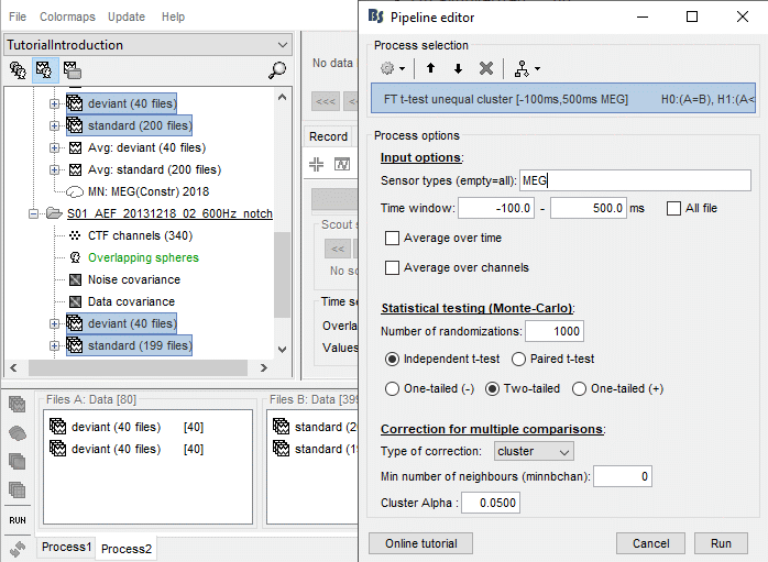
• Run the process "Test > FieldTrip: ft_timelockstatistics", Type of correction = cluster
  Note that it may require more than 5Gb of RAM and take more than 20min: check the Matlab command window for the FieldTrip progress report.
  
  

• Double-click on the new file, add a 2D topography to is (CTRL+T). Note that in the Stat tab, the options for multiple comparisons corrections are disabled, because the values saved in the file are already corrected, you can only change the significance threshold.

• Instead, you get a list of significant clusters, which you can display separately if needed. The colored dots on the topography represent the clusters, blue for negative clusters and red for positive clusters. You can change these colors in the Stat tab. Note that the clusters have a spatio-temporal extent: at one time point they can be represented as two separate blobs in the 2D topography, but these blobs are connected at other time points.
  
  

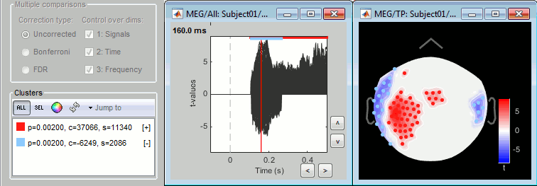
• Additional options are available for exploring the clusters, try them all. Values used to represent the clusters: p=p-value, c=cluster statistic (maxsum), s=cluster size (connected data points).
  
  

• Don't spend too much time exploring the clusters: In the previous cases, all the tests at each sensor and each time point were computed independently, we could report, individually, whether each of them was significant or not. On the other hand, the cluster-based approach just allows us to report that the two conditions are different, without specifying where or when, which makes the visual exploration of clusters relatively useless. Make sure you read this recommendation before reporting cluster-based results in your publications.

Example 4: Parametric test on sources

We can reproduce similar results at the source level. If you are using non-normalized and non-rectified current density maps, their distributions across trials should be normal, as illustrated earlier with the histograms. You can use a parametric t-test to compare the two conditions at the source level.

• Keep the same files selected in Process2. Select the button [Process sources] on both sides.

• Run the process "Test > Parametric test: Independent", Select all the data, do not average.
  Use scouts: No. When this option is not selected, it uses the entire cortex instead.
  
  

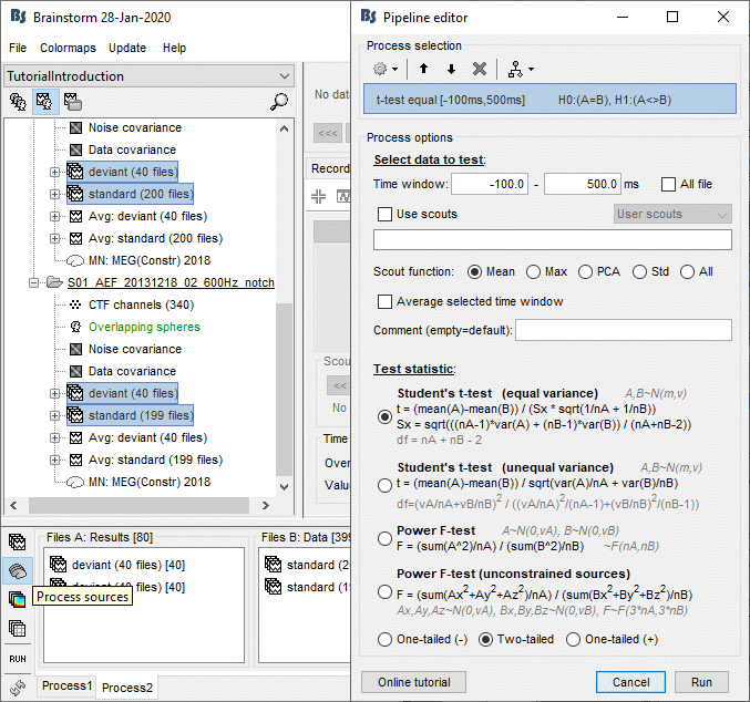
• Double-click on the new file. Change the colormap definition to show only positive values (right-click > Colormap: Stat2 > Uncheck: Absolute values) and use a different colormap ("hot" or "jet"). The sign of the relative t-statistic is not meaningful, it depends mostly on the orientation of the dipoles on the cortex (see tutorial: Difference).
  
  

Scouts and statistics

• From the Scout tab, you can also plot the scouts time series and get a summary of what is happening in your regions of interest. Non-zero values indicate the latencies when at least one vertex of the scout has a value that is significantly different between the two conditions. The values that are shown are the averaged t-values in the scout. The figure below shows the option "Values: Relative" to match surface display, but absolute values would make more sense in this case.
  
  

Unconstrained sources

There are some additional constraints to take into consideration when computing statistics for source models with unconstrained orientations. See the corresponding section in the tutorial Workflows.

Directionality: Difference of absolute values

The test we just computed detects correctly the time and brain regions with significant differences between the two conditions, but the sign of the t statistic is useless, we don't know where the response is stronger or weaker for the deviant stimulation.

After identifying where and when the responses are different, we can go back to the source values and compute another measure that will give us the directionality of this difference:
abs(average(deviant_trials)) - abs(average(standard_trials))

• Keep the same files selected in Process2. Select the button [Process sources] on both sides.

• Run process "Test > Difference of means", with the option "Absolute value of average".
  
  

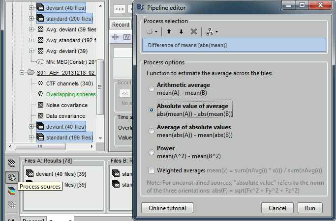
• Double-click on the new file. Double-click on the colorbar to reset it to its defaults. The sign of this difference is meaningful: red values mean "higher amplitude for the deviant condition", blue values mean "higher amplitude for the standard condition", but we don't know if they are statistically significant.
  
  

• The example above shows the two files at 148ms. The left figure shows the result of the t-test (significant effects but ambiguous sign) and the right figure shows the difference of absolute values (meaningful sign, but no statistical threshold). The superposition of the two information shows that there is some significant increase of activity in the frontal region for the deviant condition, but a decrease around the auditory cortex. This can be combined more formally as explained below.

• In Process2: FilesA = t-test results (sources), FilesB = difference deviant-standard (sources).

• Run process: Test > Apply statistic threshold, significance level α=0.01, correction=FDR.
  
  

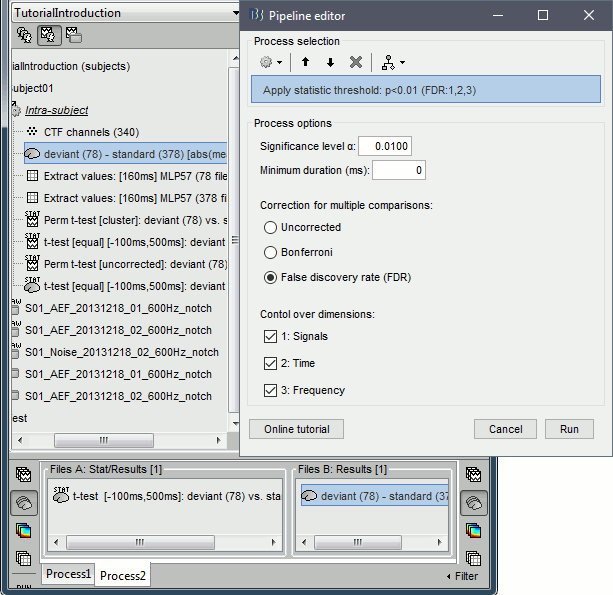
• Double-click on the new file, go to 148ms. The statistic threshold from the t-test file was applied to the difference of rectified averages (deviant-standard): only the values for which there is a significant effect between the two conditions are kept, all the others are set to zero and masked. We observe areas colored in white where the two conditions have equal amplitudes but different signs. Note that for displaying this file correctly, you must keep the amplitude slider at 0% (in the Surface tab): a correct statistic threshold is already applied to the source map, you should not perform any additional random amplitude threshold on it.
  
  

Example 5: Parametric test on scouts

The previous example showed how to test for differences across the full source maps, and then to extract the significant scout activity. Another valid approach is to test directly for significant differences in specific regions of interest, after computing the scouts time series for each trial.

This alternative has many advantages: it can be a lot faster and memory-efficient and it reduces the multiple comparisons problem. Indeed, when you perform less tests at each time point (the number of scouts instead of the number of sources), the FDR and Bonferroni corrections are less conservative and lead to higher p-values. On the other hand, it requires to formulate stronger hypotheses: you need to define the regions in which you expect to observe differences, instead of screening the entire brain.

• In Process2, select all the deviant trials (A) and standard trials (B). Select [Process sources].

• Run process Test > Parametric test: Independent, Use scouts: A1L, IFGL, M1L.
  
  

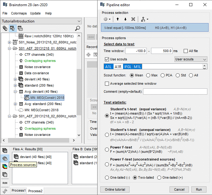
• Double-click on the new file. It shows the time points where the scout signals (averaged across vertices) are significantly different in the two conditions. We cannot represent this new file over the cortex because we have restricted the test to the scouts and discarded all the spatial information. As explained in the previous examples: the significant differences are correctly detected but the sign of the t-statistic is ambiguous.
  
  

Convert statistic results to regular files

Apply statistic threshold

You can convert the results of a statistic test to a regular file. It can be useful because lots of menus and processes are not accessible for the files with the "stat" tag display on top of their icon.

• In Process1: Select the results for the test you ran on scouts time series (example #5).

• Run process: "Test > Apply statistic threshold": α=0.01, correction=FDR, dim=[all].
  
  

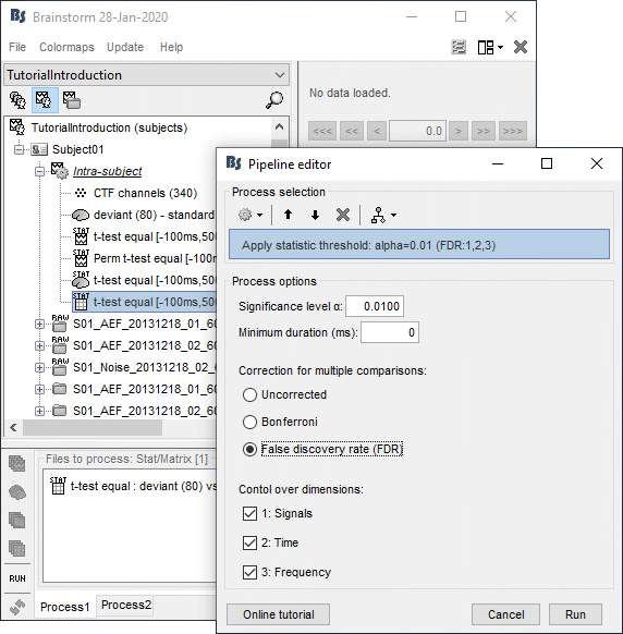
• It produces a new file with the same name but without the "stat" tag. This file is a regular matrix that you can use with any process. When you open it, the Stat tab doesn't show up.

• Note that when using this process from the Process1 tab, with one single stat file in input, the values saved in the file are the t-values from the stat file, not the original physical units. In order to obtain real physical units, you need to call the process with two inputs: the stat file on the left, and the file with the values of interest on the right, as in the previous section Directionality: Difference of absolute values.

Simulate recordings from these scouts

• Compute a head model for the intra-subject folder:
  Right-click on the channel file > Compute head model, keep all the default options.
  Note that this channel file was created during one of the processes involving the two runs, it contains an average of their respective channel files (average head positions).

• In Process1, select the new thresholded matrix file.

• Run process: "Simulate > Simulate recordings from scout", select option Save full sources.
  
  

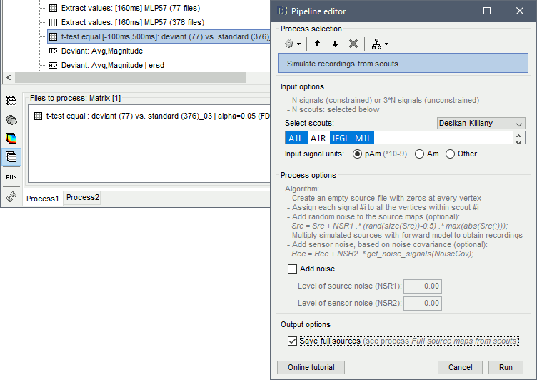
• This process creates two files. First it maps the scouts time series on the cortex: it creates an empty source file with zeroes everywhere, then for each scout it maps the values of the input time times series to the sources within the ROI. Then it multiplies these artificial source maps with the forward model to simulate MEG recordings.
  
  

• Note that this example is not adapted to simulate realistic MEG values. The source time series used in input for the process "Simulate recordings from scouts" are t-values, and not realistic physical units for a current source density (in pAm). The simulated MEG values localize correctly the simulated scouts, but with meaningless amplitudes. For realistic simulations, you must use input signals with amplitudes that correspond to minimum norm current density maps (in pAm). You can obtain these e.g. by computing them with process "Extract > Scout time series".

Example 6: Nonparametric test on time-frequency maps

Two run a test on time-frequency maps, we need to have all the time-frequency decompositions for each individual trial available in the database. In the time-frequency tutorial, we saved only the averaged time-frequency decompositions of all the trials.

• In Process1, select all the trials from both conditions and both runs.

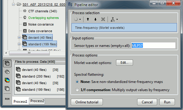
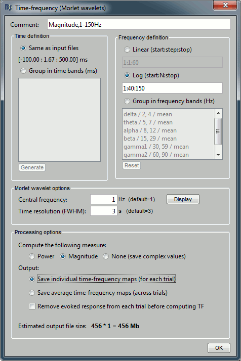
• Run process "Frequency > Time-frequency (Morlet wavelets)". Select the options as below.
  Select only one sensor (eg. MLP57) to make it faster. Save individual TF maps.
  Measure=Magnitude: It is more standard to test the square root of power (amplitude).
  Do not normalize the TF maps for a test within a single subject (only for group studies).
  
  

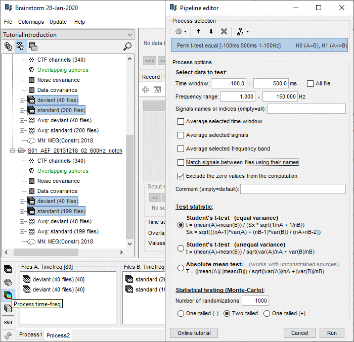
• In Process2, select all the deviant trials (A) and standard trials (B). Select [Process time-freq].

• Run process: Test > Permutation test: Independent, 1000 randomizations, no correction.
  No need to select the option "Match signals between files" because the list of signals is the same for all the trials. If you have marked bad channels in some trials during your analysis, you would need to select this option.
  
  

• Double-click on the new file. In the Stat tab, select α=0.05 uncorrected.
  
  

• If you run this test on time-frequency files where the power has been saved, you get this warning:
  
  

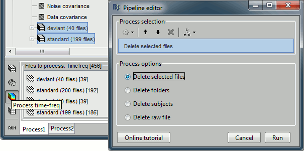
Now delete the TF decompositions for the individual trials:

• In Process1, select the files for which you computed the TF decomposition (all trials).

• Select the [Process time-freq] button.

• Run process: File > Delete files, option Delete selected files.
  
  

Export to SPM

An alternative to running the statistical tests in Brainstorm is to export all the data and compute the tests with an external program (R, Matlab, SPM, etc). Multiple menus exist to export files to external file formats (right-click on a file > File > Export to file).

Two tutorials explain how to export data specifically to SPM:

• Export source maps to SPM8 (volume)

• Export source maps to SPM12 (surface)

On the hard drive

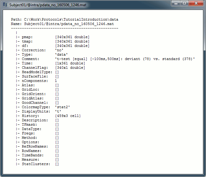
Right click on the first test we computed in this tutorial > File > View file contents.

• 

Description of the fields

• pmap: [Nsignals x Ntime x Nfreq]: p-values for all the data points. If empty, computed from tmap:
  pmap = process_test_parametric2('ComputePvalues', tmap, df, TestType, TestTail);

• tmap: [Nsignals x Ntime x Nfreq]: t-values for all the data points.

• df: [Nsignals x Ntime x Nfreq]: Number of degrees of freedom for each test.

• Correction: Correction for multiple comparison already applied ('no', 'cluster', 'fdr', ...)

• Type: Initial type of the data ('data', 'results', 'timefreq', 'matrix').

• Comment: String displayed in the database explorer to represent the file.

• The other fields were copied from the files that were tested, and were described previously.

Useful functions

• process_test_parametric2: Two-sample independent parametric t-test

• process_test_parametric2p: Two-sample paired parametric t-test

• process_test_parametric1: One-sample parametric t-test (against zero)

• process_ttest_baseline: One-sample parametric t-test (against baseline)

• process_ft_timelockstatistics: FieldTrip tests for recordings (file type "data")

• process_ft_sourcestatistics: FieldTrip tests for source maps (file type "results")

• process_ft_freqstatistics: For time-frequency and scouts (file type "timefreq" and "matrix")

• Conversion Brainstorm to FieldTrip: out_fieldtrip_data, out_fieldtrip_results, out_fieldtrip_timefreq, out_fieldtrip_matrix

• process_extract_pthresh: Computes the pmap from the tmap, and saves thresholded files.

• process_test_parametric2('ComputePvalues', t, df, TestType, TestTail)

• bst_stat_thresh: Computes the Bonferroni and FDR corrections in Brainstorm.

Additional documentation

Articles

• Bennett CM, Wolford GL, Miller MB, The principled control of false positives in neuroimaging
  Soc Cogn Affect Neurosci (2009), 4(4):417-422.

• Maris E, Oostendveld R, Nonparametric statistical testing of EEG- and MEG-data
  J Neurosci Methods (2007), 164(1):177-90.

• Maris E, Statistical testing in electrophysiological studies
  Psychophysiology (2012), 49(4):549-65

• Bennett CM, Wolford GL, Miller MB, The principled control of false positives in neuroimaging
  Soc Cogn Affect Neurosci (2009), 4(4):417-422.

• Pantazis D, Nichols TE, Baillet S, Leahy RM. A comparison of random field theory and permutation methods for the statistical analysis of MEG data, Neuroimage (2005), 25(2):383-94.

• Kiebel SJ, Tallon-Baudry C, Friston K
  Parametric analysis of oscillatory activity as measured with EEG/MEG, HBM 2005

• FieldTrip video: Non-parametric cluster-based statistical testing of MEG/EEG data:
  https://www.youtube.com/watch?v=vOSfabsDUNg

Related tutorials

• Machine learning: Decoding / MVPA

Forum discussions

• Multiple comparisons: http://neuroimage.usc.edu/forums/showthread.php?1297

• Cluster neighborhoods: http://neuroimage.usc.edu/forums/showthread.php?2132

• Differences FieldTrip-Brainstorm: http://neuroimage.usc.edu/forums/showthread.php?2164

• Statistics on sources: https://neuroimage.usc.edu/forums/t/11876

• Citing the non-parametric tests in an article: https://neuroimage.usc.edu/forums/t/non-parametric-or-parametric-stats-implemented-in-brainstorm/24907/5

• Conjunction inference: https://neuroimage.usc.edu/forums/t/common-source-activation-across-subjects-and-conditions/1152

• Normalize PSD based on resting-state before statistical tests: https://neuroimage.usc.edu/forums/t/psd-normalization-based-on-the-resting-psd/37854

---