Hi @sugata_hisato,
The difference is in how coherence is estimated, this is a detailed description of the two methods:
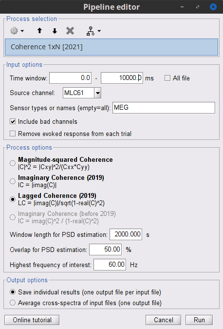
A. Connectivity > Coherence [2021] > Lagged Coherence
This process obtains only one coherence spectrum estimate using all the windows
These 2 parameters control how coherence is computed:
-
Time window: This refers to the part of the signal that you want to analyze, often All file is often selected.
-
Window length for PSD estimation: Time window to compute the xy-CrossSpectrum, and the x- y-AutoSpectra (which are the same to their PSDs). These spectra are used to compute coherence. Overlap for PSD estimation: This parameter controls the number of windows that will be used to estimate the coherence spectra in the current segment.
Coherence (C) is computed as the ratio of the xy-CrossSpectrum, and the x- y-AutoSpectra
For example with these parameters:
- Time window: 0 -10,000 ms
- Lagged coherence
- Window length for PSD estimation: 2000 ms
- Overlap for PSD estimation: 50% (250 ms)
If the input is one file, and Output option is Save individual results... :
- The first 10 s of signal are split in 9 windows of 2 s, with 1 s overlap. One xy-CrossSpectrum, and two AutoSpectra (one for x and one for y) are computed for each window.
- Then, xy-CrossSpectrum, and two AutoSpectra are averaged across windows.
- The Coherence spectrum is computed using the averaged CrossSpectrum and averaged AutoSpectra. Thus there is one Coherence spectra for the 10-s signal
4.Finally, lagged coherence is then computed from C as LC = |imag(C)| / sqrt(1 - real(C)^2)
If the input are multiple files, and Output option is Average cross-spectra..., one Coherence spectrum is obtained from the averaged (across all windows in all files) xy-CrossSpectrum and AutoSpectra
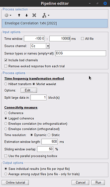
B. Connectivity > Envelop correlation [2022] > Lagged Coherence
Computing coherence through the "envelope correlation" process, is a bit different, as there is one coherence spectrum estimate for each window
These 3 parameters control how coherence is computed:
-
Time window: This refers to the part of the signal that you want to analyze, often All file is often selected.
-
Time resolution:
- Dynamic (one coherence estimate per window)
- Static (average coherence spectrum across windows)
-
Estimation window length: Time window to compute the xy-CrossSpectrum, and the x- y-AutoSpectra (from the TF representations). Sliding window overlap: This parameter controls the number of windows.
Coherence (C) is computed as the ratio of the xy-CrossSpectrum, and the x- y-AutoSpectra
For example with these parameters:
- Time window: 0 -10,000 ms
- Morlet wavelet: 1:1:40 Hz
- Lagged coherence
- Time resolution: Dynamic
- Estimation window length 2000 ms
- Sliding window overlap 50% (1000 ms)
If the input is one file, and Output option is Save individual results... :
- A TF representation is obtained using the Morlet wavelet approach (40 frequencies)
- The TF map is then split in nine windows of 2 seconds each, with 1 second overlap
- For each window, CrossSpectrum and AutoSpectra are computed using all the time samples in the window (nTimeSamples = estimation_window_length * fs)
- Then a Coherence spectrum is computed for each window, thus there are a total of nine Coherence spectra for the 10-s signal
5.Finally, lagged coherence is then computed from C as LC = |imag(C)| / sqrt(1 - real(C)^2)
Note: The Static time resolution option performs the average of the lagged coherence, and not the average of the CrossSpectrum and AutoSpectra (as it is done in Coherence [2021])
If the input are multiple files, and Output option is Average cross-spectra..., the previous steps are executed for each file, and the result is averaged across files.
Best,
Raymundo


