Source model average looks unexpectedly messy

[jamluijten]

Hi Brainstorm,

I want to do a group analysis on source models, but I worry I am doing something wrong. I have some questions on averaging source models and scouts time series.

Some background: I am doing an analysis on somatosensory evoked potentials (SEPs) in MEG data. I used the default anatomy for my subjects and warped the anatomy for each of them. For this question, I am looking at surface source models.

First, I averaged my epochs based on the SEP triggers for each separate session (sensor average). Then, as I am using the default anatomy, I used Unconstrained source estimation for all sensor averages (Settings: Compute sources [2018]. Minimum norm imaging, Current density map, Unconstrained, MEG sensors.). (As I am working with MEG data, I used overlapping spheres (surface) as head models.)

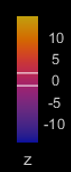
According to the Workflows tutorial (https://neuroimage.usc.edu/brainstorm/Tutorials/Workflows#Unconstrained_cortical_sources) for group analysis, the next step for a group analysis is to normalize (z-score) the current density source maps for all subjects w.r.t. baseline. I did this with the Process1 box (Process sources > Standardize > Baseline normalization. Baseline 200 to 5 ms before SEP trigger. Z-score). Next, I flattened the cortical maps (Process sources > Sources > Unconstrained to flat map. Norm). After this, I selected the normalized and flattened source models I wanted to average and dragged them into Process1. I used Process sources > Average > Average files > Everything. I used 'Everything' as I only dragged the source maps I wanted to average into the Process1 box.

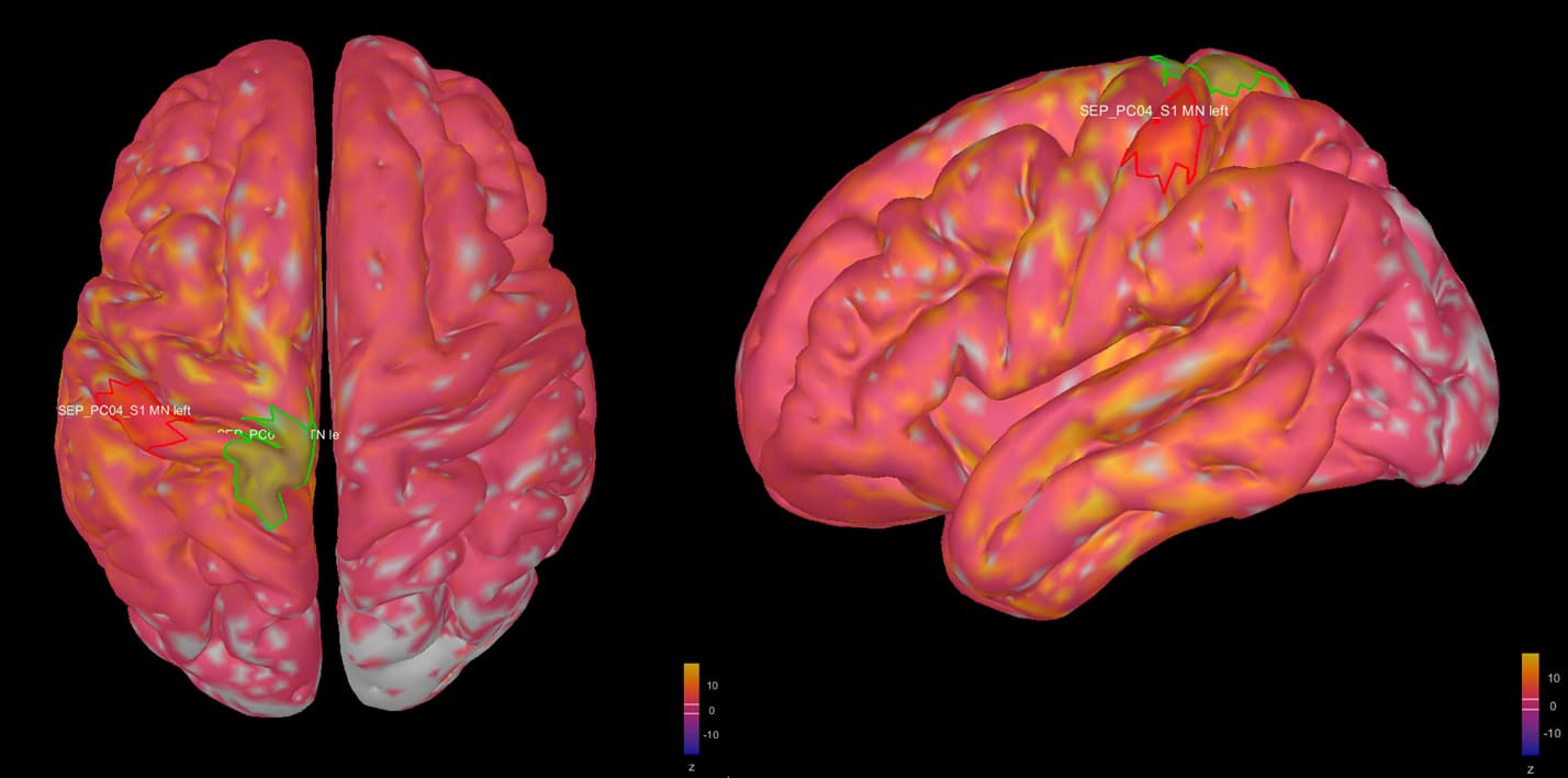
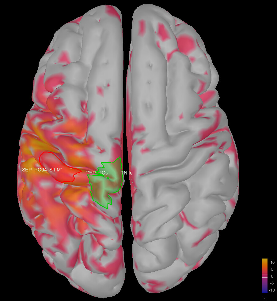
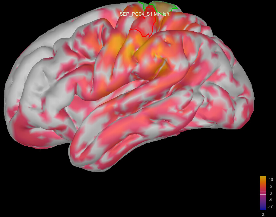
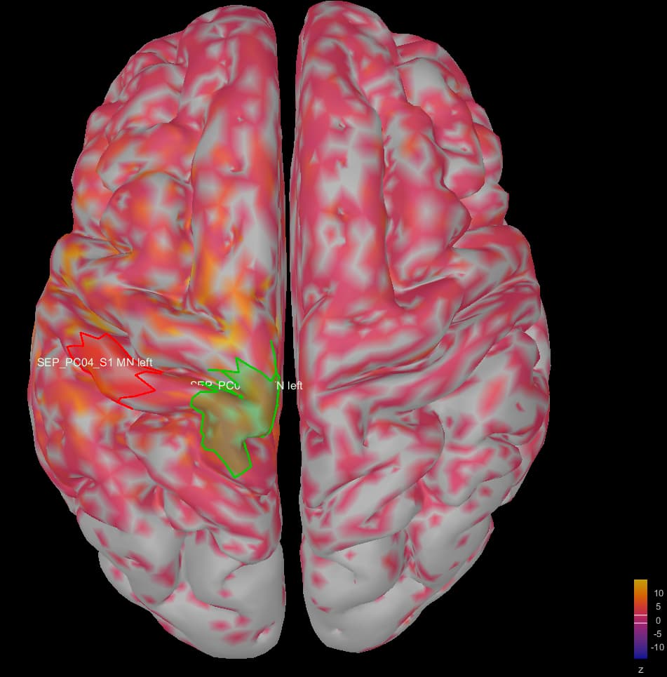
This is where I was surprised: the average source model looks very messy and speckled, whereas the individual source models of my subjects looked very clean. Next to this, the focus of activity that I am expecting in the primary somatosensory cortex (like in my individual subject's source models) has spread/leaked onto almost the entire left hemisphere. I included some images below for clarity.
Is this something you see more often, and is it just part of averaging source models, or did I do something wrong here? Can it be caused by the warning I receive when averaging the source models ("The channels files from the different studies do not have the same number of channels. Cannot create a common channel file")? Should I fix this by creating a uniform channel file?

My last question is on averaging scouts time series. In case this is just the way my averaged source models will look, it is not useful for visualization of the averages and it might be better to just average my subject's scouts time series directly. So: is averaging source models and extracting the scouts time series from the average source model equal to extracting the scouts time series from subject's source models and average these scouts time series myself?

Please let me know if I need to clarify my question(s) any further. And of course, thanks in advance for helping me!

Best,
Janne

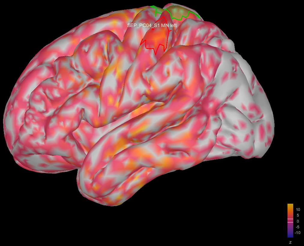
Image 1: the individual source maps of my subjects (n=4), all normalized and flattened, at t=27 ms

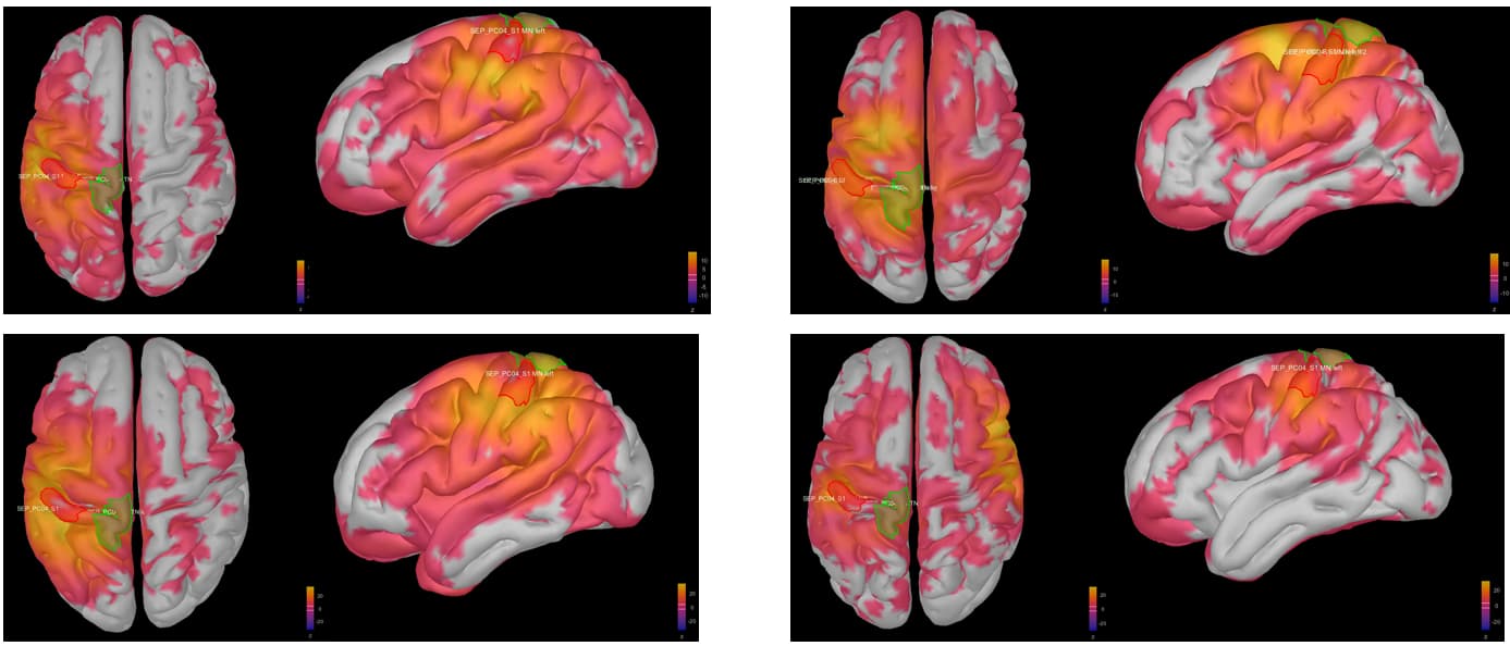
Image 2: my average source map of these subjects, at t=27 ms as well. They are not smoothed, smoothing did not make things better.

[Raymundo.Cassani]

Hi Janne,

@jamluijten

I used 'Everything' as I only dragged the source maps I wanted to average into the Process1 box.

This is correct.

For sake of completeness: averaging source maps like this (without projection to Default anatomy) only applies sources from Subjects using the Default anatomy or using warped Default anatomy. This is because the warped anatomies have the same number of vertices (as the Default one), and there is a correspondence of one-to-one with the Default anatomy.

https://neuroimage.usc.edu/brainstorm/Tutorials/CoregisterSubjects#Warped_brains

@jamluijten

This is where I was surprised: the average source model looks very messy and speckled, whereas the individual source models of my subjects looked very clean.

It is hard to see in the attached image, it seems the range of the z-scores varies greatly among subjects.

Is that the case?
Was this also observed in the average evoked fields?
Did you try with constrained sources?

@jamluijten

Can it be caused by the warning I receive when averaging the source models ("The channels files from the different studies do not have the same number of channels. Cannot create a common channel file")? Should I fix this by creating a uniform channel file?

This warning can be disregarded. The channel files are not being used.
Moreover, the source files are already co-registered.

@jamluijten

So: is averaging source models and extracting the scouts time series from the average source model equal to extracting the scouts time series from subject's source models and average these scouts time series myself?

Yes, they are the same if using default and/or warped anatomies, and if the Scouts:

• are extracted on the flattened source maps
• use the Scout function mean
• are defined with the same vertices for each Subject

mean_over_vertices(mean_over_subjects(sources) === mean_over_subjects(mean_over_vertices(sources)

[jamluijten]

Hi Raymundo,

Thank you for the fast response! It's really helpful.

Yes, the z-scores do vary among subjects. The ranges on the exact images are (in the same order):

However, if I average the top 2 subjects and the bottom 2 subjects separately, I get similar results (spreading of activity and spottiness).

I'm sorry, what do you mean by the average evoked fields? Do you mean my scout signal? I did not try to average them separately yet. Should I?

Perhaps this answers your question a bit: In the average, my scouts time series were also 'spreaded' compared to the individual maps. With this, I mean that in my individual maps, the scouts time series on the S1 hand area had higher SEP amplitudes compared to the S1 foot area after stimulation of the hand area, as can be expected. In the averaged source map, both scouts time series had similar amplitudes, which does not really make sense to me. It does match the image of widespread activation of the entire left hemisphere rather than an activation focus, which is the issue here (in my opinion).
Do you by any chance have an explanation for this?

I did try with constrained sources, that made things worse in terms of messyness (visually). I know this is due to the orientation of the sources perpendicular to the cortex. Images below are all made at the same time point again (t=27 ms).

This is an example of the subject at the top left of the image in my previous post:

As you can see, the individual source map looks messy already. However there still is local activation that I would expect.

The average (of all 4 subjects again) looked like this:

The activation spread to the entire hemisphere again.

It's very good to know that I can disregard the channels warning.
And thank you for clarifying when averaging source models is equal to averaging scouts directly, that is also very helpful to know! To be complete, I suppose that flattening of the source maps should be done using Norm and not PCA for this to be true?

Best,
Janne

[Sylvain]

Hello Janne,

I recommend you first flatten the maps then compute the Z-scores in each individual before you average. If the sign of the activation does not matter to your study, I would even recommend that you flatten then take the absolute value of the time series before computing the individual z-scores and group averaging.

[jamluijten]

Hi Sylvain,

Thank you for helping me. If you don't mind me asking, why would you recommend deviating from the step-by-step plan described in the 'Workflows' tutorial by flattening (using Norm?) first and computing z-scores afterwards?

And I'm sorry, I don't entirely understand taking the absolute values after flattening. Does flattening not always result in positive values as it's the square root of squares? Or do you mean flattening by PCA in these recommendations?

Over all, are these recommendations meant for source estimation models, or scouts time series, or both?

Best,
Janne

[Sylvain]

Sorry Janne: I didn't catch that you had used the norm for flattening. Then my suggestion of exploring the effect of taking the absolute value is moot. The issue seems to be with group averaging then. Can you produce intermediate averages including 2, then 3 and finally the 4 subjects in the average and check where this starts to break?

[jamluijten]

Hi Sylvain,

No problem!

Would you recommend PCA over Norm for flattening?

And why would you recommend to first flatten the maps and then compute Z-scores in the individual maps? I did this the other way around, according to the 'Workflows' tutorial. Should I change this?

I tried averaging with 2 subjects that had similar z-scores (top 2 and bottom 2 of my first post), but this caused spreading of activation onto the entire hemisphere as well, even though the individual maps had focused activation in S1 (at a certain point in time, of course).

[Raymundo.Cassani]

@jamluijten

I'm sorry, what do you mean by the average evoked fields?

I meant to examine the MEG recordings to verify that the noise levels across participants.

@jamluijten

I tried averaging with 2 subjects that had similar z-scores (top 2 and bottom 2 of my first post), but this caused spreading of activation onto the entire hemisphere as well, even though the individual maps had focused activation in S1 (at a certain point in time, of course).

You may want to low-pass filter the evoked responses to compensate for the different latencies in each subject:
https://neuroimage.usc.edu/brainstorm/Tutorials/VisualGroup#Subject_averages:_Filter_and_normalize

[jamluijten]

Hello Sylvain and Raymundo,

Thank you both for taking the time to reply and help me.

However, I am getting a little confused as the recommendations in this thread do not align with the Brainstorm tutorials, so I don't understand why one or the other would be better for my case.

Could you perhaps provide some clarity on the following matters?

1. In which case is the rule stated below true? Is it if I use PCA for flattening, or if I use Norm for flattening, or both? Is this still true if I introduce (low-pass) filtering?

@Raymundo.Cassani

Yes, they are the same if using default and/or warped anatomies, and if the Scouts:

• are extracted on the flattened source maps
• use the Scout function mean
• are defined with the same vertices for each Subject

mean_over_vertices(mean_over_subjects(sources) === mean_over_subjects(mean_over_vertices(sources)

2. You both seem to assume that I use PCA for flattening. Why is this? Is PCA recommended over Norm? In the Workflows tutorial, Norm is mentioned so I thought Norm should be used. Is this incorrect/not commonly used?

3. What would be the advantage of flattening first, and then using z-score normalization? Why should I do this instead of the order stated in the Workflows tutorial (Workflows/Unconstrained_cortical_sources)?

4. I understand that low-pass filtering would compensate for different latencies. However, low-pass filtering also skewers the z-score normalization leading to an overestimation of z-scores. Should I filter after z-score normalization?

5. My issue is not exactly differences in latencies, as my average scouts signals look ok. I do have peaks around points in time I would expect. My issue is this unexpected spreading of activity in the source estimation model onto the entire left hemisphere. I drew a scout on the temporal lobe, and it's time series is approximately the same as my S1 hand area, which is just not physically possible. Is this something I could resolve by filtering?

6. Could this image of scattered activation be caused by head motion of one of the subjects?

I hope you can help me,

Thank you in advance,
Janne

PS:

@Raymundo.Cassani

I meant to examine the MEG recordings to verify that the noise levels across participants.

The noise levels in my sensor averages were in the same range.

[jamluijten]

Hi Brainstorm,

Some background: I am doing an analysis on somatosensory evoked potentials (SEPs) in MEG data. I imported warped anatomies for my subjects from another protocol using the same subjects. I want to do a surface analysis as well as a volume analysis. With averaging source models, I noticed some issues.

I posted a question on messy average source models this week (Source model average looks unexpectedly messy), and I think I figured out where the discrepancy is coming from. My question is now: how to solve this issue?

I figured it out by copying one subject, and then averaging one source estimation model and it's direct copy. Displayed on the group analysis cortex, this led to a very messy and spreaded/speckled activation as described in my previous topic. To figure the problem out, I loaded the three .mat source files into Matlab, and checked the ImageGridAmp matrices in the 2 identical individual source maps and for the average. This ImageGridAmp matrix was identical for all 3. This told me that the problem was not in averaging itself. The only difference I could detect was the 'SurfaceFile', being _warped for the individual source maps and default for the group analysis average. Looking into these surface files, the Cube grids differed. This told me that the combination of ImageGridAmp and SurfaceFile was what went wrong in my protocol.

The warped anatomies I imported used, I suppose, the ICBM152 2019 default anatomy. The grid is 197x233x489. The default anatomy in my protocol is ICBM152 2023b, using a 193x229x193 grid.

I think I can solve this issue through two routes:

1. I can keep 'my' default anatomy (2023b), and project all individual warped anatomies to this default anatomy. This fixes the projection on the brain visually if I open the source file in the group analysis. However, this does change the ImageGridAmp matrix. For the abovementioned example, this meant that the average was not identical to the two copy's anymore. I do not know if this really changes the values of averaging, or just changes the rows (vertices) of the ImageGridAmp. Also, I don't know the consequences for my volume analysis. I created a group analyis volume source grid before doing head models and volume source estimation. I suppose this grid is now based on 'my' 2023 default anatomy, so volume source averaging might be ok this way.

2. Use the 2019 default anatomy, so change the default anatomy in my protocol. I don't know the full consequences of this route as well. Changing the default anatomy means that averaging my warped anatomy surface source models goes well in terms of the ImageGridAmp matrix as well as the display on the volume analysis cortex model. However, I don't know if this raises problems for the volume analysis I want to after this. I suppose I need to create a new group analysis volume source grid and do volume source estimation again. Will this fix the issue?

Please let me know if you have any questions, I did some more experiments that led me to these two route options.

Edit: I don't think the default anatomy really matters for volume source averaging, as I have to do "Project source grid" before averaging either way. It looks ok after doing that both on the 2023 anatomy and in a backup-protocol I used to try changing to the 2019 anatomy. Could this be correct?

What route would you recommend, and why? What should I look out for when performing the routes? What steps in the analysis should I re-do?

Thank you in advance for helping me,

Best regards,
Janne

[Raymundo.Cassani]

Correct, if there is projection, anatomies can be different.

@jamluijten

I figured it out by copying one subject, and then averaging one source estimation model and it's direct copy. Displayed on the group analysis cortex, this led to a very messy and spreaded/speckled activation as described in my previous topic. To figure the problem out, I loaded the three .mat source files into Matlab, and checked the ImageGridAmp matrices in the 2 identical individual source maps and for the average. This ImageGridAmp matrix was identical for all 3.

Thanks for the detailed exploration! You got the issue, the Default anatomy in Protocol and the Default anatomy that was warped are not the same. The problem is not exactly the difference in the MRI cube. But the difference in their cortical surfaces. While these surfaces have the same same number of vertices, vertex order may be different (e.g., vertex 1000 in one surface is in a different place than vertex1000 in the other surface) , i.e. there is not a correspondence one-to-one, then the spotted plots. The one-to-one correspondence is assumed when working with warped anatomies.

When you do projection, the issue is addressed as a correspondence that is not-one-to-one is computed between surfaces. The average in the projection is different, as it transformation between surface is computed. E.g, in the resulting surface, activity vertex 1000, may be the combination of the activity of vertices in the original surface. It is not likely that is only a "change the rows (vertices)" as there is not a one-to-one correspondence.

@jamluijten

Edit: I don't think the default anatomy really matters for volume source averaging, as I have to do "Project source grid" before averaging either way.

It will not matter, as projection will compute correspondence between volumes.

@jamluijten

What route would you recommend, and why? What should I look out for when performing the routes? What steps in the analysis should I re-do?

Route 1. Ideally, in the Protocol the warped anatomies should be the default anatomy in protocol warped. This has as advantage that there is nor need of projection, so going from warped to default anatomy does not take time. Also warped anatomies will not be default warped anatomies, but another-anatomy warped, this will introduce (great) confusion.

Route2. This makes more sense than Route1. Although, you would need to assure that default anatomy in protocol is exactly the same that was used in the warped ones, otherwise, you will have the initial problem.

P.S. I merged the posts

[jamluijten]

Thank you for the detailed explanation. If you don't mind, I have some small follow-up questions to verify that I solve this problem the best way possible.

@Raymundo.Cassani

Thanks for the detailed exploration! You got the issue, the Default anatomy in Protocol and the Default anatomy that was warped are not the same. The problem is not exactly the difference in the MRI cube. But the difference in their cortical surfaces. While these surfaces have the same same number of vertices, vertex order may be different (e.g., vertex 1000 in one surface is in a different place than vertex1000 in the other surface) , i.e. there is not a correspondence one-to-one, then the spotted plots. The one-to-one correspondence is assumed when working with warped anatomies.

I'm happy to hear that this is indeed the issue, explaining the speckled source maps.

@Raymundo.Cassani

When you do projection, the issue is addressed as a correspondence that is not-one-to-one is computed between surfaces. The average in the projection is different, as it transformation between surface is computed. E.g, in the resulting surface, activity vertex 1000, may be the combination of the activity of vertices in the original surface. It is not likely that is only a "change the rows (vertices)" as there is not a one-to-one correspondence.

I indeed figured it was something like this, as my scouts time series differed very slightly in amplitude. It is good to know the reasoning behind it, thank you. This answer also tells me that "Route 1" is not recommended, which is good to know as well.

As I understand correctly, I should do the following:

1. Verify that the default anatomy that was used for warping is indeed the ICBM152 2019 version.
2. If so, change the default anatomy in my protocol. Is this the correct manner?: Go to anatomy view. Right-click 'Default anatomy' > Use template > MNI > ICBM152_2019.
3. Fix volume analysis:
   3.1 Re-calculate a Group Analysis Volume Source Grid, as I suppose this Source Grid is based on the default anatomy? Or is this not necessary (I'm sorry, I don't fully understand the answer regarding the volume source averaging)
   3.2 Do head models and source estimation again for my volume models.
4. Do nothing for my surface models, as averaging them is okay now (warped anatomy and default anatomy align).

Does this fix my issue? Am I missing something? Should I re-do more steps in my analysis, or less?

Thank you so much for helping me solve this issue.

Best,
Janne

[Raymundo.Cassani]

The steps look good.

Double (triple) check Step 1. E.g, Once you change the Default anatomy, create a FakeSubject01, import the channels and warp, compare the vertices XYZ coordinates (Vertices field in SurfaceFile) with Subject01, they MUST be the same. Also, you can do the average with itself test.

[jamluijten]

Thank you. So I do need to redo the volume analysis after I change the default anatomy?

I have another idea:
I imported warped anatomies from another protocol, let's call this Protocol A.
Is it a good option to copy the '@default_subject' folder from Protocol A's "anat" folder to my protocol's "anat" folder directly through File Explored on my laptop? This way, it is definitely the correct default anatomy, right?

@Raymundo.Cassani

compare the vertices XYZ coordinates (Vertices field in SurfaceFile) with Subject01, they MUST be the same

Thank you for the test suggestion. I wonder though, are the vertices XYZ coordinates not dependent on how I warp the anatomy? If I use slightly different orientation, does it change the XYZ coordinates?

[Raymundo.Cassani]

@jamluijten

So I do need to redo the volume analysis after I change the default anatomy?

TLDR: No, but you would need to create a Template grid to aggregate data from different subjects:
https://neuroimage.usc.edu/brainstorm/Tutorials/CoregisterSubjects#Volume_source_models

Projecting for Volume and Surface sources is dealt a bit different. In Surface, the dipoles are located at the vertices of the a Surface mesh, then the projection of warped to default is only one-to-one. For Volume sources, the location of the dipoles is not based points (vertices) of the anatomy, but in the points of a grid that is produced by filling the cortical surface, this means different surfaces, different grids. So, to aggregate across subjects a template grid is defined; then when computing sources for a subject, the coordinates of all the points in the template grid are converted to the subject space and sources are computed, all subjects have now the same number of sources in locations that are equivalent.

@jamluijten

Is it a good option to copy the '@default_subject' folder from Protocol A's "anat" folder to my protocol's "anat" folder directly through File Explored on my laptop? This way, it is definitely the correct default anatomy, right?

That should do the trick.

• Close Brainstorm and Matlab before copy/pasting the files.
• Copy/paste rather than Move in case an error happens

@jamluijten

Thank you for the test suggestion. I wonder though, are the vertices XYZ coordinates not dependent on how I warp the anatomy? If I use slightly different orientation, does it change the XYZ coordinates?

Yes, it is dependent. My comment was considering that warping was done without manual intervention (e.g, only with head points)

[jamluijten]

Hi Raymundo,

Thanks for the confirmation on how to copy the default anatomy!
I'll be careful with copy/paste.

@Raymundo.Cassani

TLDR: No, but you would need to create a Template grid to aggregate data from different subjects:

Yes, I'm aware of this process. I made a template grid for my volume models before. I'm just wondering if I should redo the Template grid after I change the default anatomy. Maybe I'm wrong, but I thought this template grid is based on the default anatomy. If this is correct, it means that my current Template grid is based on the 2023 default anatomy. And so, after copying the 2019 default anatomy from Protocol A to my protocol, I guess I should create the Template grid again?
(And consequently, redo head models and source estimation using this new grid)

[Raymundo.Cassani]

Yes, you need to redo the template grid with the new default anatomy, and re estimate sources for each subject with the new template grid.

[jamluijten]

Thank you! It's super clear now.

Thanks for all your help in this issue!