I am working on 120 seconds of resting state data and am seeing if there are any activation differences at certain ROIs. I have 14 controls and 18 OCD patients. I chose ROIs based on the Destrieux atlas (32 of them) consisting of areas like orbital frontal cortex, the cingulate gyrus as well as some areas in the prefrontal cortex. I realize that the most common type of analysis for resting state data is time frequency, coherence etc. When I did F-test on the extracted scouts from source data with constrained orientation and averaged across time, I got really high F-values. When I view it in table mode, it shows the numbers are on the order of 100,000s but when I view it in time series view it shows it at like 12. Also, when I do the same thing using scouts from unconstrained source data, I get null results.
This is my process for constrained sources:
Compute sources using sLORETA(constrained) -> Extract scout time series -> Run parametirc test Independent (with all patient scouts in A and controls in B): Select option Average time and F-test.
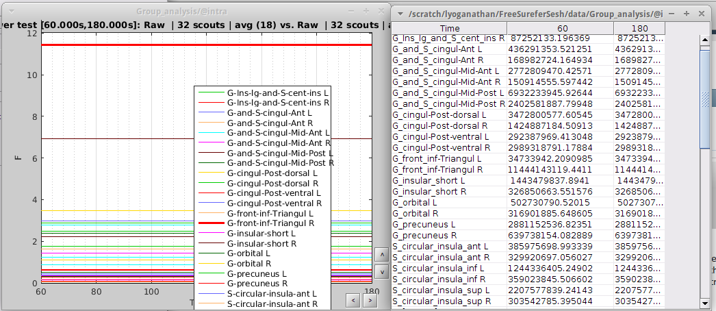
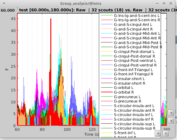
I got F values in the range of 100000s. (see image for table vs time series). If I average before running the test (Process -> Average-> Average time on all scout files), i get the same results so no problem there. But if you look at what it looks like not averaged across time, we see the highest peak with about f value of 45. To me, it dosen't make sense that just by averaging, the F values can go so high. I tried with and without flipping the sign and got similar results. However with t-test on the average across time data everything becomes null.
Compute sources using sLORETA(unconstrained) -> Extract scout time series(with option unconstrained orientation:norm) -> Run parametirc test Independent (with all patient scouts in A and controls in B): Select Option average time and F test.
I get mostly null, some things approach significant (at p=0.17 uncorrected) when averaged across time. When I don't average, the data looks similar to the constrained across time results, with random peaks.
The option i used for both scenarios was the power F test - test as well average time window. Why are the results so different between constrained unconstrained when I average across time?
You have one block of two minutes of resting recordings for each subject and you want to test the differences between two groups of subjects, right?
I don’t think that any of the approaches you present here are adapted to this type of data.
With your current pipeline, if you do not average over time, it tests for differences for each time point independently. But why would you expect the values at a given time point (eg. t=60s) to be significantly higher in one group or another? To compare ongoing recordings (not stimulus-driven), you need first to compute a metric that integrates the time.
This is what you’ve been trying to do by averaging in time, but this is not a good solution either. If your recordings are long enough, the average in time of the oscillating signals you record will tend to zero. The constrained sources are oscillating signals (the sign of the signal is preserved) and would also tend to zero. The unconstrained sources (with a norm applied, like you did), will tend to a strictly positive value related with the average power of the signal. Your two measures are completely unrelated, one tests the mean, the other tests the variance. Hence the very different results you get between constrained and unconstrained sources.
What you should do instead is to compute some power metric in frequency space (for instance a PSD measure) for your entire time window. You can keep the full spectrum or group the values by frequency bands (the former is more indicated in the case of a group study). Then you can test the power in one frequency band between your two groups. This is applicable to both constrained and unconstrained sources. I would recommend you compute this for the entire brain first, and then refine by region of interest if the effects you observe are not significant with the full brain.
Before going further with this new option, I would recommend you start by doing a literature review to identify some metrics of interest related with the effects your are interested in. You will not be able to explore your dataset and compute any meaningful statistic without a clear hypothesis (eg. the group A shows a stronger power in a specific frequency band and a specific brain region).
One additional note about your current pipeline: Do not extract the scouts manually, use the scout selection in the process options instead. It will avoid many manipulation errors, will produce more accurate results and in many cases it will be faster.
Indeed, most if not all papers on resting state data look at frequencies or use functional connectivity measures.
I've been going through the literature on resting state oscillatory brain dynamics, which seems kind of interesting. Usually they do FFT on epochs of data from the resting state recordings. I've pulled some quotes from some papers:
All participants had at least 45 s of artifact-free data...To transform MEG data from the time domain into the frequency domain, a Fast Fourier Transform (FFT) was applied to artifact-free two-second epochs of continuous data for each of the two orthogonally oriented time series at each regional source. Each two-second epoch overlapped 50% with the next epoch, and each epoch was multiplied by a cosine squared window. This combination of overlap and windowing ensured that each time point contributed equally to the mean power spectra. The mean power spectra for the two orthogonally oriented time series at each regional source were summed to yield the power at a given frequency at that source
-Lauren Cornew, Timothy P. L. Roberts, Lisa Blaskey, J. Christopher Edgar.(2012) Resting-State Oscillatory Activity in Autism Spectrum Disorders. Journal of Autism and Developmental Disorders, 42, 1884. doi:10.1007/s10803-011-1431-6
Two approximately 13 s long artifact free epochs (sample rate 312.5 Hz; 4096 samples) were selected for further analysis... Relative band power was computed for the two 13 s epochs in the following frequency bands: 0.5–4 Hz (δ), 4–8 Hz (θ), 8–13 Hz (α), 13–30 Hz (β) and 30–48 Hz (γ). Results of the two epochs were averaged for each subject.
-J.L.W. Bosboom, D. Stoffers, C.J. Stam, B.W. van Dijk, J. Verbunt, H.W. Berendse, E.Ch. Wolters. (2006) Resting state oscillatory brain dynamics in parkinson's disease: An MEG study. Clinical Neurophysiology 117, 2521-2531. doi:10.1016/j.clinph.2006.06.720
It seems it is okay to take epochs of the resting state data per participant and average them, the compute stats using the averages. Was wondering if in your opinion this is a good approach? Why not just compute PSD of FFT over the entire time domain? And what would be a good time window for each epoch?
Use all the time available to compute the PSD/Welch, and define the estimator window to get the frequency resolution you are interested in.
Longer estimator window = more frequency bins = less windows averaged together = more noise