|
Size: 9308
Comment:
|
← Revision 20 as of 2022-03-15 14:28:32 ⇥
Size: 7068
Comment:
|
| Deletions are marked like this. | Additions are marked like this. |
| Line 1: | Line 1: |
| = Export source maps to SPM12 = The statistical analysis is still limited in Brainstorm, but you can easily export your source maps and run your tests with an external application. This tutorial explains how to export source maps to SPM12. It is based on the median nerve tutorial dataset that was used in the tutorials of the section [[Tutorials/TutRawViewer|Processing continuous recordings]]. If you have followed those tutorials, this dataset should be available in your database in the protocol '''!TutorialRaw'''. |
= Export surface source maps to SPM12 = ''Authors: Francois Tadel'' The statistical analysis is still limited in Brainstorm, but you can easily export your source maps and run your tests with an external application. This tutorial explains how to export source maps to SPM12. It is based on the older introduction tutorials ([[Tutorials/MedianNerveCtf|CTF median nerve stimulation]], protocol TutorialRaw), but it is easy to translate it to the new tutorials (auditory oddball). SPM12 can work with source activations represented either as '''volumes''', as illustrated in the tutorial [[ExportSpm8|Export to SPM8]], or as '''surfaces''', as presented in this tutorial. |
| Line 6: | Line 10: |
| == Calculate unconstrained sources == In the previous tutorial, we have calculated sources constrained to the cortex surface. Because SPM8 works only with full volumes, we are going to estimate the sources in the full head volume, as detailed in the tutorial [[Tutorials/TutVolSource|Volume source estimation]]. |
== Export source files == We want to export the sources estimated for all the trials for the '''left '''condition to surface files in GIfTI format (readable by SPM). We are going to get rid of the time information because it cannot be represented in SPM, and keep only two averaged time windows per condition: a baseline '''[-20,-15]ms''' and an active state '''[33,38]ms'''. |
| Line 9: | Line 13: |
| Right-click on (common files) > Compute head model > MRI volume. | Clear the Process1 box and drop all the trials for condition Left in it. Select the button "Process sources" on the left of the Process1 tab. |
| Line 11: | Line 15: |
| {{attachment:unconstrHeadmodel.gif||height="239",width="432"}} | {{attachment:introBst.gif||width="438",height="364"}} |
| Line 13: | Line 17: |
| Right-click on the new head model > Compute sources > keep all the default options. | Select the process "File > Export to SPM12 (surface)". |
| Line 15: | Line 19: |
| {{attachment:unconstrSources.gif||height="227",width="387"}} Pick any of the unconstrained source file and drop it in the Process1 box. Run the process "Standardize > Z-score (dynamic)". It creates a new shared source file, available for all the files of Subject01. {{attachment:zscored.gif||height="259",width="473"}} == Export source files == We want now to export the z-scored unconstrained sources to volume files in NIfTI1 format (readable by SPM). We are going to get rid of the time information, very difficult to handle with those full volumes in SPM, and keep only two averaged time windows per condition: a baseline [-20,-15]ms and an active state [33,38]ms. We are going to generate 2*101 left + 2*98 right .nii files. Clear the Process1 box and drop all the trials for condition Left in it. Select the button "Process sources" on the left of the Process1 tab. To select only the unconstrained/z-scored files, you could simply use the checkbox "zscore", but we are going to illustrate a more generic solution: select the process "File > Select files with tag" (detailed in the tutorial [[SelectFiles|Selecting files in the database]]). Configure it as following: {{attachment:selectFiles.gif||height="307",width="478"}} Then in the same pipeline, select the process "File > Export to SPM". {{attachment:exportLeftBaseline.gif||height="319",width="307"}} |
{{attachment:exportLeftBaseline.gif||width="310",height="241"}} |
| Line 34: | Line 23: |
| * '''Output folder''': Select the folder where you want all the .nii files to be saved * '''Output file tag''': Set the file name to this exported .nii files. If you leave this option empty, the default file names would be "Subject01_Left_*.nii", which is not informative enough, given that we want to export two states for the same condition: baseline vs. active. * '''Time window''': Segment of the file that we want to export. We start with the baseline: -20ms to -15ms * '''Time downsample factor''': If we keep the time information, we can save only one time sample every N in the .nii files, to limit the size of the generated files. The value we set here is not used because we specify in the last option that we average in the time dimension. * '''Volume downsample''': Set it to 3, it will take one voxel every three voxels in each dimension. The MRI volume we imported in the Brainstorm database is 256x256x256, the output volumes with the functional data are only 86x86x86, again to limit the size of the files we generate at this step. * '''Average over time''' / '''Keep time dimension''': Defines what we do with the time. In this case, we want to average over the small time windows to get rid of the time. |
* '''Output folder''': Select the file format of the output files (choose "GIfTI-1 (*.gii)"), the select the folder where you want all the .gii files to be saved. * '''Output file tag''': Set the file name of the exported .gii files. If you leave this option empty, the default file names are "SubectName_Condition_*.gii", which in this case would be "Subject01_Left_*.gii". This is not informative enough, given that we want to export two states for the same condition: baseline vs. active. Set this option it manually to "subject01_left_baseline". * '''Average time window''': Segment of the file that we want to export and average in time. We start with the baseline: -20ms to -15ms * '''Use absolute values of the sources''': If this option is selected, the source amplitudes will be all positive instead of positive and negative. This is usually a better way to represent the activation of a brain area, and better adapted for statistical analysis in SPM. |
| Line 41: | Line 28: |
| Add another export process right after this one, to export the "active" state. Set the time window to [33,38]ms, to capture the peak of the response in the primary somatosensory cortex, and the file name to "subject01_left_active". | Add another export process after this one, to export the "active" state. Set the time window to [33,38]ms, to capture the peak of the response in the primary somatosensory cortex, and the file name to "subject01_left_active". |
| Line 43: | Line 30: |
| {{attachment:exportLeftActive.gif||height="343",width="309"}} | {{attachment:exportLeftActive.gif||width="311",height="261"}} |
| Line 45: | Line 32: |
| Click on Run and let it process for a while. It will generate 2*101=202 NIfTI files in the output folder. | Click on Run and let it process for a while. It will generate the following files (total of '''12 Mb'''): |
| Line 47: | Line 34: |
| Repeat the operation for the right condition: change only the file output names to "subject01_right_baseline" and "subject01_right_active". | * Subject01_cortex.gii: Contains the definition of the cortex surface (faces and vertices) * subject01_left_active_*.gii: 101 files, definition of the trials for the active condition * subject01_left_active_*.dat: 101 files, actual source maps for the active condition * subject01_left_baseline_*.gii: 101 files, same for the baseline condition * subject01_left_baseline_*.dat: 101 files, same for the baseline condition |
| Line 49: | Line 40: |
| {{attachment:exportRightActive.gif||height="344",width="309"}} | This representation is quite heavy (405 files) for so little information. Hopefully this will get improved in a future release of SPM12. |
| Line 51: | Line 42: |
| Open you file explorer and check the .nii files that were created in the destination folder. {{attachment:allNii.gif}} You can try opening some of those files with a NIfTI file viewer, just to make sure that what is saved is coherent. You can use for instance the free software [[http://www.mccauslandcenter.sc.edu/mricro/mricron/|Mricron]] to view the file subject01_right_active_02.nii. This a stimulation of the right median nerve, we can see clearly that the response is located in the central regions of the left hemisphere, which is what we expect. {{attachment:mriCron.gif||height="342",width="286"}} Note that you can also you Brainstorm as a NIfTI viewer: go to the anatomy view of the protocol, right-click on Subject01 > Import MRI > Select a .nii file. == Export T1 MRI == One last thing we need to export from Brainstorm: the T1 MRI volume of the subject, on which we would like to see the results in SPM. Go the anatomy view of the protocol !TutorialRaw, right click on Subject01 / MRI > File > Export to file. Select the file format "MRI: NIfTI-1" and save the file '''T1.nii''' in the same folder with all the other .nii files. {{attachment:exportMri.gif||height="264",width="348"}} == Run SPM == Installing SPM is easy: http://www.fil.ion.ucl.ac.uk/spm/software/spm8/ |
== Run SPM12 == Installing SPM is easy: [[http://www.fil.ion.ucl.ac.uk/spm/software/spm8/|http://www.fil.ion.ucl.ac.uk/spm/software/spm12/]] |
| Line 71: | Line 47: |
| {{attachment:spmStart1.gif||height="170",width="276"}} | '''Import note''': Do not run Brainstorm and SPM at the same time, always close Brainstorm before starting SPM (but you don't need to close Matlab). {{attachment:spmStart1.gif||width="276",height="170"}} |
| Line 75: | Line 53: |
| {{attachment:spmStart2.gif||height="329",width="285"}} | {{attachment:spmStart2.gif||width="285",height="329"}} |
| Line 79: | Line 57: |
| * '''Directory''': Select the folder in which the results to be saved, for instance create a sub-folder "spm" in the folder in which you have saved all the NIfTI files. | * '''Directory''': Select the folder in which the results to be saved, for instance create a sub-folder "spm" in the folder in which you have saved all the GIfTI files |
| Line 81: | Line 59: |
| * '''Group 1 scans''': Select all the post-stim trials for the left condition (subject01_left_active_*.nii) * '''Group 1 scans''': Select all the pre-stim trials for the left condition (subject01_left_baseline_*.nii) |
* '''Group 1 scans''': Select the 101 post-stim files '''subject01_left_active_*.gii''' * '''Group 2 scans''': Select the 101 pre-stim files '''subject01_left_baseline_*.gii''' |
| Line 88: | Line 66: |
| {{attachment:spmSetupTwoSample.gif||height="656",width="493"}} | Once you have defined all the options, click on the '''Run '''button (the green button in the toolbar on top of the Batch Editor window). |
| Line 90: | Line 68: |
| Once you have defined all the options, click on the '''Run '''button (the green button in the toolbar on top of the Batch Editor window). The design matrix window is displayed in the Graphics window, and a file SPM.mat is saved in the output directory you defined in the options. | {{attachment:spmSetupTwoSample.gif||width="493",height="656"}} |
| Line 92: | Line 70: |
| {{attachment:spmDesign.gif||height="505",width="447"}} | The design matrix window is displayed in the Graphics window, and a file '''SPM.mat''' is saved in the output directory you defined in the options. |
| Line 94: | Line 72: |
| In the SPM8 Menu window, click on the '''Estimate''' button. Select the SPM.mat file that was just created. SPM estimates the parameters, it may take a while. | {{attachment:spmDesign.gif||width="341",height="511"}} |
| Line 96: | Line 74: |
| {{attachment:spmRun.gif||height="185",width="241"}} | In the SPM12 Menu window, click on the '''Estimate''' button. Select the '''SPM.mat''' file that was just created. SPM estimates the parameters, it may take a while. |
| Line 98: | Line 76: |
| When done click on '''Results''' in the SPM8 Menu window, select again the same SPM.mat file. A window pops up, you have to specify the contrast(s) of interest. | {{attachment:spmRun.gif||width="241",height="185"}} |
| Line 100: | Line 78: |
| {{attachment:spmContrast1.gif||height="285",width="338"}} | When done click on '''Results''' in the SPM12 Menu window, select again the same '''SPM.mat''' file. A window pops up, you have to specify the contrast(s) of interest. |
| Line 102: | Line 80: |
| Click on "t-constrasts" and "Define new constrast...". Edit the options to define the t-test post-stim > pre-stim: | {{attachment:spmContrast1.gif||width="338",height="285"}} Click on "Define new contrast...". Edit the options to define the t-test post-stim > pre-stim: |
| Line 105: | Line 85: |
| * '''Type''': t-constrast | * '''Type''': t-contrast |
| Line 109: | Line 89: |
| {{attachment:spmContrast2.gif||height="282",width="335"}} | {{attachment:spmContrast2.gif||width="335",height="282"}} |
| Line 113: | Line 93: |
| {{attachment:spmContrast3.gif||height="282",width="333"}} | {{attachment:spmContrast3.gif||width="333",height="282"}} |
| Line 115: | Line 95: |
| Click on "Done", then a list of parameters is asked in the "SPM8: Stats: Results" window. | Click on "Done", then a list of parameters is asked in the "SPM12: Stats: Results" window. |
| Line 120: | Line 100: |
| * '''p-value (FWE)''': 0.05 | * '''p-value (FWE)''': 0.01 |
| Line 124: | Line 104: |
| {{attachment:spmContrast4.gif||height="224",width="308"}} | {{attachment:spmContrast4.gif||width="324",height="335"}} |
| Line 126: | Line 106: |
| Then the typical SPM8 glass brain shows up in the Graphics window. The window SPM8 Results shows more display options for this figure. Select "'''overlays > sections'''". Pick the file '''T1.nii''' we exported from Brainstorm. | You get the final results in the Graphics window. You can click on the cortex surface to rotate. |
| Line 128: | Line 108: |
| {{attachment:spmContrast5.gif||height="214",width="327"}} You get the final results in the Graphics window. You can explore the volume by clicking on the MRI slices. {{attachment:spmResults.gif||height="461",width="307"}} |
{{attachment:spmResultsConstr.gif||width="432",height="338"}} |
| Line 137: | Line 113: |
<<EmbedContent(http://neuroimage.usc.edu/bst/get_feedback.php?ExportSpm12)>> |
Export surface source maps to SPM12
Authors: Francois Tadel
The statistical analysis is still limited in Brainstorm, but you can easily export your source maps and run your tests with an external application. This tutorial explains how to export source maps to SPM12. It is based on the older introduction tutorials (CTF median nerve stimulation, protocol TutorialRaw), but it is easy to translate it to the new tutorials (auditory oddball).
SPM12 can work with source activations represented either as volumes, as illustrated in the tutorial Export to SPM8, or as surfaces, as presented in this tutorial.
Contents
Export source files
We want to export the sources estimated for all the trials for the left condition to surface files in GIfTI format (readable by SPM). We are going to get rid of the time information because it cannot be represented in SPM, and keep only two averaged time windows per condition: a baseline [-20,-15]ms and an active state [33,38]ms.
Clear the Process1 box and drop all the trials for condition Left in it. Select the button "Process sources" on the left of the Process1 tab.
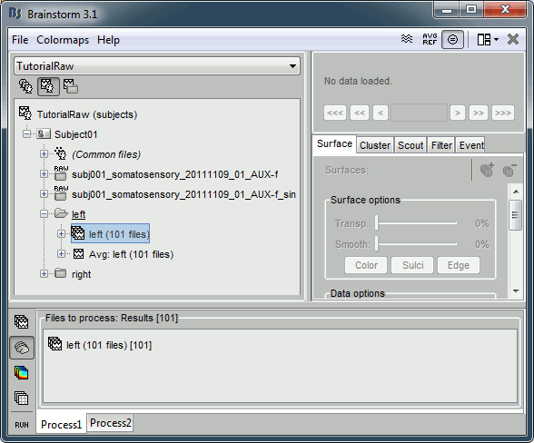
Select the process "File > Export to SPM12 (surface)".
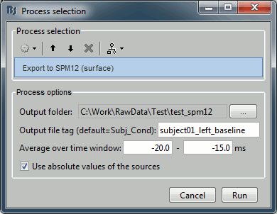
Configure the process:
Output folder: Select the file format of the output files (choose "GIfTI-1 (*.gii)"), the select the folder where you want all the .gii files to be saved.
Output file tag: Set the file name of the exported .gii files. If you leave this option empty, the default file names are "SubectName_Condition_*.gii", which in this case would be "Subject01_Left_*.gii". This is not informative enough, given that we want to export two states for the same condition: baseline vs. active. Set this option it manually to "subject01_left_baseline".
Average time window: Segment of the file that we want to export and average in time. We start with the baseline: -20ms to -15ms
Use absolute values of the sources: If this option is selected, the source amplitudes will be all positive instead of positive and negative. This is usually a better way to represent the activation of a brain area, and better adapted for statistical analysis in SPM.
Add another export process after this one, to export the "active" state. Set the time window to [33,38]ms, to capture the peak of the response in the primary somatosensory cortex, and the file name to "subject01_left_active".
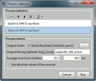
Click on Run and let it process for a while. It will generate the following files (total of 12 Mb):
- Subject01_cortex.gii: Contains the definition of the cortex surface (faces and vertices)
- subject01_left_active_*.gii: 101 files, definition of the trials for the active condition
- subject01_left_active_*.dat: 101 files, actual source maps for the active condition
- subject01_left_baseline_*.gii: 101 files, same for the baseline condition
- subject01_left_baseline_*.dat: 101 files, same for the baseline condition
This representation is quite heavy (405 files) for so little information. Hopefully this will get improved in a future release of SPM12.
Run SPM12
Installing SPM is easy: http://www.fil.ion.ucl.ac.uk/spm/software/spm12/
Start Matlab, go to the SPM folder, add it to your path if it is not done already, then type "spm". Select "M/EEG" on the SPM startup screen.
Import note: Do not run Brainstorm and SPM at the same time, always close Brainstorm before starting SPM (but you don't need to close Matlab).
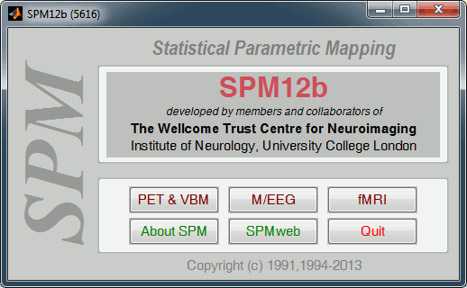
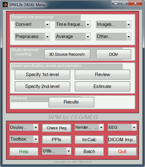
In the main SPM window, click on "Specify 2nd level".
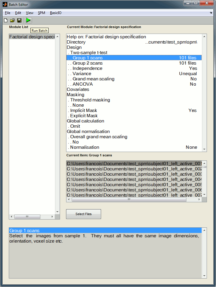
Now you can specify your stats design in the Batch Editor window. We are going to start with a simple t-test for the left condition: active state versus baseline. Select the following options:
Directory: Select the folder in which the results to be saved, for instance create a sub-folder "spm" in the folder in which you have saved all the GIfTI files
Design: Two sample t-test
Group 1 scans: Select the 101 post-stim files subject01_left_active_*.gii
Group 2 scans: Select the 101 pre-stim files subject01_left_baseline_*.gii
Independence: Yes
Variance: Unequal
Grand mean scaling: No
ANCOVA: No
Once you have defined all the options, click on the Run button (the green button in the toolbar on top of the Batch Editor window).
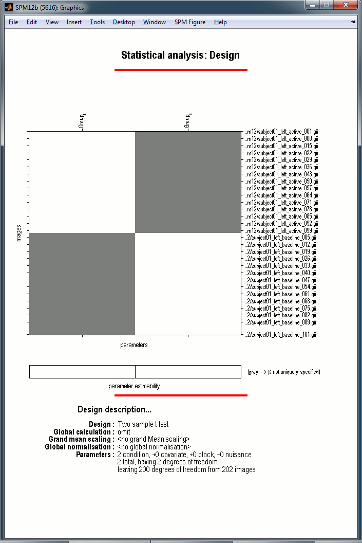
The design matrix window is displayed in the Graphics window, and a file SPM.mat is saved in the output directory you defined in the options.
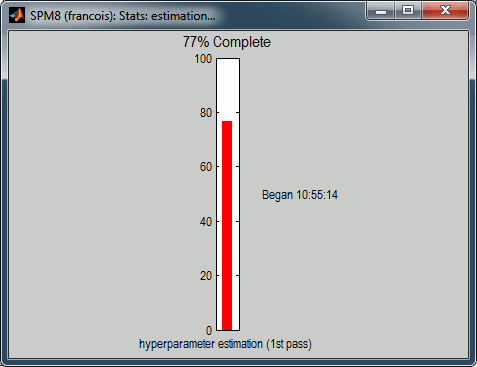
In the SPM12 Menu window, click on the Estimate button. Select the SPM.mat file that was just created. SPM estimates the parameters, it may take a while.
When done click on Results in the SPM12 Menu window, select again the same SPM.mat file. A window pops up, you have to specify the contrast(s) of interest.
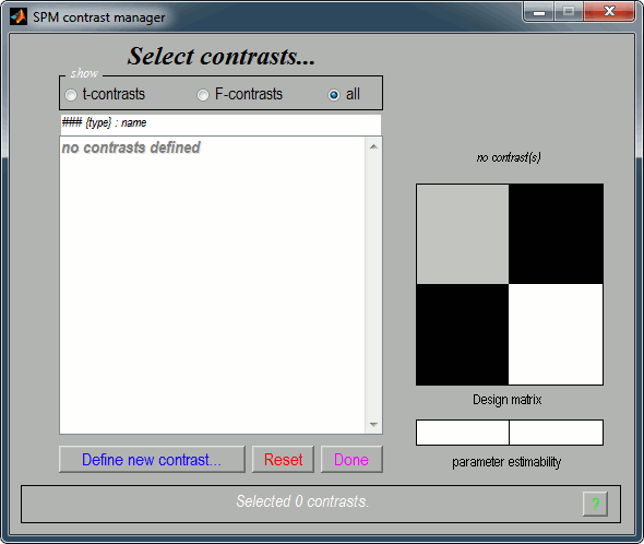
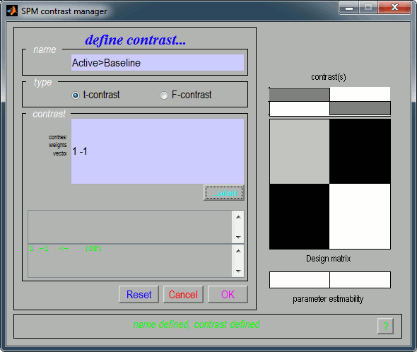
Click on "Define new contrast...". Edit the options to define the t-test post-stim > pre-stim:
Name: Give a name to the contrast, for display. Enter for instance "Active>Baseline".
Type: t-contrast
Contrast: Enter "1 -1" to test for "Group1 (active files) > Group2 (baseline files)"
- Click on "...submit" to update the figure, then "Ok" to add the new contrast.
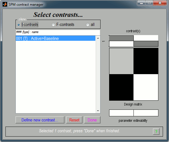
It updates the window "SPM contrast manager".
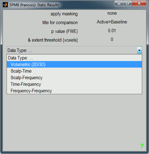
Click on "Done", then a list of parameters is asked in the "SPM12: Stats: Results" window.
Apply masking: None
Title for comparison: "Active>Baseline" for instance
p-value adjustment to control: FWE (=Family-Wise Error, to correct for multiple comparisons)
p-value (FWE): 0.01
& extent threshold (voxels): 0
Data type: Volumetric (2D/3D)
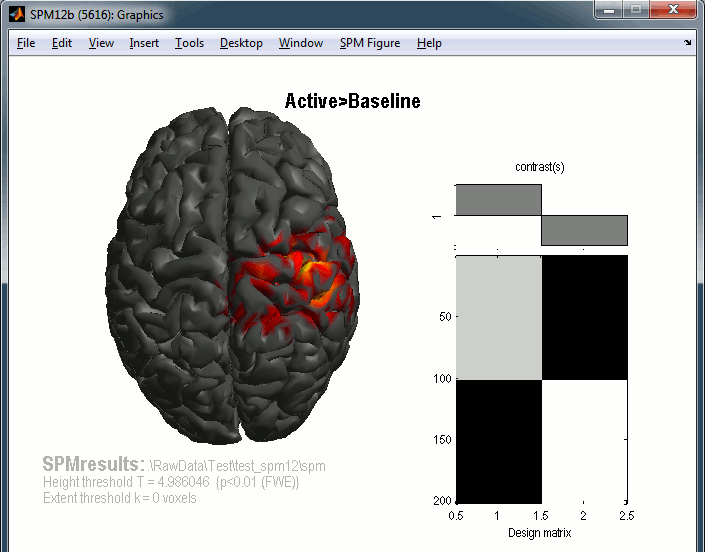
You get the final results in the Graphics window. You can click on the cortex surface to rotate.
You can repeat the same operations with the right condition.
The results you get here are very basic, but the logic of exporting source results from Brainstorm to SPM can be extended to any type of analysis.
