DBA tutorial: Compute sources in deep cerebral structures

Authors: Jean-Eudes Le Douget, Francois Tadel, Denis Schwartz, Raymundo Cassani

This tutorial explains step-by-step how to use the DBA (Deep Brain Activity) functionality, useful to assess subcortical source localization.

Warnings: (added in April 2021)

1. The mixed head models introduced in this tutorial are complicated to handle in terms of data structures, they produce values of different types in the same files, and have shown to cause many interpretation and computation errors among Brainstorm users. For general studies, we recommend using simpler source spaces: surface or volume.

2. Mixed head models are mostly indicated for individual subject analysis, and not suitable for group analysis when using individual anatomy for all the subjects. We do not have any accurate solution for projecting the individual mixed source space to the template space. use volume head models instead. See tutorials: Volume source estimation, Subjects coregistration.

Import database

This tutorial is based on resting-state recordings for 7 subjects with two conditions: eyes open (YO), eyes closed (YF). We have recorded 20 runs of 15 seconds for each subject and each condition.

The goal is to compute the contrast between the two conditions in the alpha band. The data has already been filtered in the alpha frequency band (7-13Hz) and the default anatomy is used for all the subjects.

• Start by downloading the tutorial dataset TutorialDba.zip from the Download page.

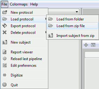
• The file is an exported Brainstorm protocol. To load it in your database, use the menu:
  File > Load Protocol > Load from zip file.
  
  

Select deep structures

The first step consists in creating the surface file that includes the cortex and the deep structures that we want to include in the model. Here, in the default anatomy:

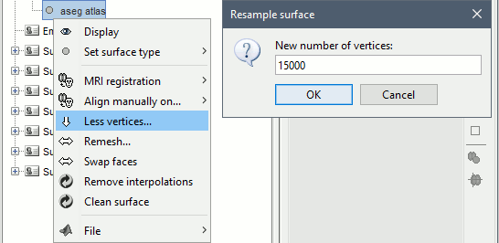
• Right-click on "aseg atlas" > Less vertices > 15000 vertices. Use the default resmpling method (Matlab's reducepatch) for now.
  
  

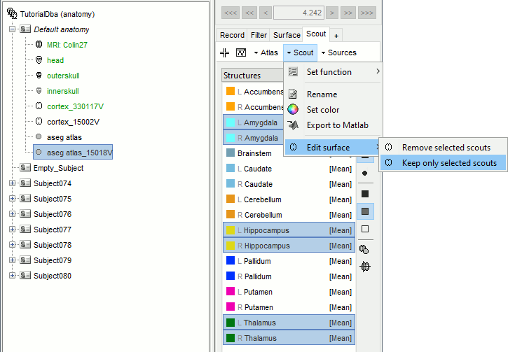
• Double-click on "aseg atlas_15018V" (contains the subcortical structures from the FreeSurfer altas). Don't worry if the final number of vertices is slightly different than the one specified.

• Select the amygdala, the thalamus and the hippocampus, and create a subatlas.
  
  

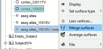
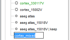
• Merge the cortex with the selected structures. Rename the new surface in "cortex_mixed".
  
  

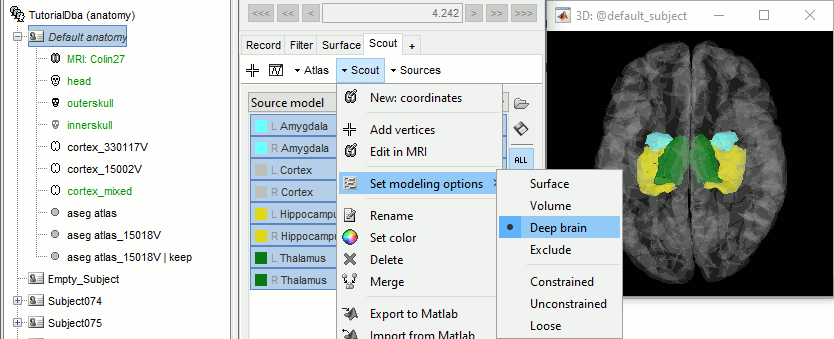
• Open the cortex_mixed surface and create a new atlas "Source model options". With Matlab 2015b+, the display looks weird because it limits the number of possible transparent layers to 5. To produce nicer figures, disable the OpenGL renderer (File > Edit preferences). The display will be much slower, but the renderer won't suffer from this limitation.
  
  

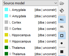
• Select all the structures and set modeling options to "Deep brain" for all of them.
  
  

• It will automatically set the orientation constraint to "constrained" for the cortex and hippocampus regions, and "unconstrained" for all the other regions. Don't forget to close the window with the new surface so that all these changes can be saved.
  
  

Location and orientation constraints

Two types of constraints can be applied to each anatomical region in the atlas "Source model":

• Location constraint: Defines where the sources corresponding to these regions are placed.

  • Surface: The sources are located on the surface of the structure (cortex and hippocampus). The surface describing the region is directly used as the source space.

  • Volume: The sources are located inside the volume of the region. The source space is a grid of points uniformly distributed inside of the volume delimited by the surface of the structure.

  • Deep brain: Use the preferred configuration defined in the Deep Brain Atlas (surface for the cerebral cortex and hippocampus, volume for all the other structures).

• Orientation constraint:

  • Constrained: Defines only one dipole per grid point, with a fixed orientation orientation.

    • With option "Surface": Uses the normal orientation to the surface at each point.
    • With option "Deep brain": Uses the preferred orientation defined in the atlas (see below).

  • Unconstrained: Uses three orthogonal dipoles per grid point (x,y,z).

  • Loose: Intermediate option, uses three orthogonal dipoles per grid point, but favors the preferred orientation used for the constrained case.

Based on the anatomical observations reported for each subcortical region in the reference articles (next section), the preferred combination of constraints is described below. The reference articles also estimate the number of averaged trials needed to detect responses in some regions.

• 	Location constraint	Preferred orientation	Default orientation constraint	Trials (MEG)	Trials (EEG)
  Cortex	Surface	Normal	Constrained	-	-
  Hippocampus	Surface	Normal	Constrained	21	45
  Cerebellum	Surface	Normal	Unconstrained	-	-
  Accumbens	Volume	None	Unconstrained	-	-
  Amygdala	Volume	None	Unconstrained	-	-
  Brainstem	Volume	None	Unconstrained	400 (LGN)	490 (LGN)
  Caudate	Volume	None	Unconstrained	-	-
  Putamen	Volume	None	Unconstrained	34	23
  Pallidum	Volume	Y axis	Constrained	> 10000	> 10000
  Thalamus	Volume	None	Unconstrained	3500	3700

Source estimation

Head model

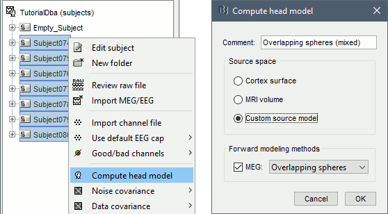
• Select all the subjects (except for the empty room recordings) > right-click > Compute head model. Select "Custom source model", and leave the other options to their defaults.
  
  

• You can explore the source grids that were computed. Right-click on one of the head models > Check source grid (volume) and Check source grid (surface). In the Scout tab, select the atlas "User scouts" to get a clearer view. In panel Surface, increase the transparency of the surface to see the source grids representing the select subcortical regions.
  
  

Inverse model

• The noise covariance matrix was estimated from the empty room recordings (Empty_Subject) and copied to all the folders of all the subjects.

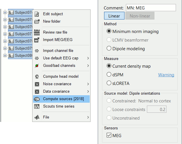
• Select all the subjects (except the empty room recordings), right-click > Compute sources.
  Select Minimum norm (wMNE) and leave the other options to their default values.
  
  

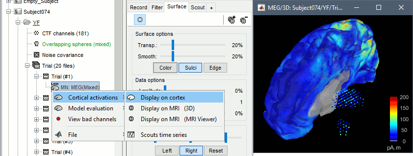
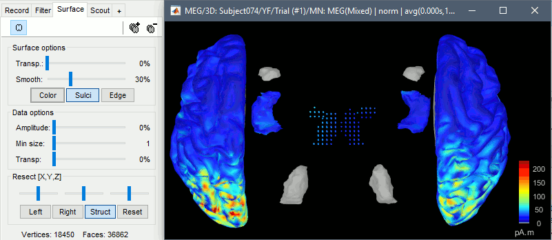
• Double-click on the sources for any trial (segment of 15s of rest recordings). Make sure the atlas "User scouts" is selected in the Scout tab, then explore the display options available in the Surface tab. The surface regions (cortex and hippocampus) are represented as surfaces, and the values are directly mapped on the surface. The volume regions (amygdala and thalamus) are represented as grids of dots.
  
  

• To be able to visualize the activity of the subcortical regions, you can use the button [Struct] at the bottom of the Surface tab. It moves the different structures so you can see them all. The grid points corresponding to the volume regions stay in place, so you can see them (while the corresponding surface is moved).
  
  

Compute statistics

We will now design a statistical analysis to assess the eyes-open and eyes-closed contrast. As a reminder, the recordings available in the database have already been filtered in the alpha frequency band (7-13Hz). As a measure of the global of the activity in this frequency band, we will average all the time samples in each block of 15s. Note that this is not the recommended procedure anymore: it would have been better to simply compute a PSD from the sources estimated for the continuous file link, but this option was not available at the time this tutorial was written.

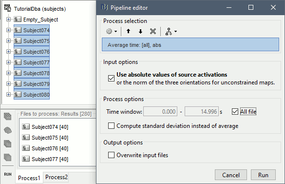
• In Process1, select all the subjects (except for Empty_Subject)and select [Process sources].

• Run process Average > Average time > Use absolute value, All file.
  
  

• The option Use absolute values of source activations also "flattened" the source maps. The regions that had a few regions with "unconstrained" source orientations, with three values per grid point. These three orientations were grouped into one value by taking the norm along the three axes: sqrt(x²+y²+z²).

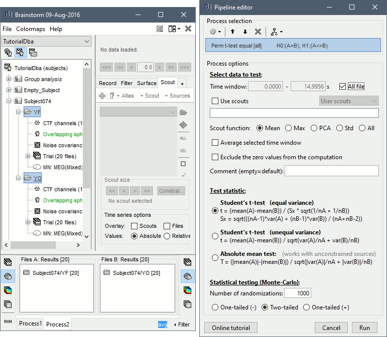
• In Process2, select FilesA=Subject74/YF (eyes closed) and FilesB=Subject74/YO (eyes open). Then enter "avg" in the Filter box, to select only the time averages. You should have 20 files selected on each side.

• Run the process Test > Permutation test (independent), as configured as below:
  
  

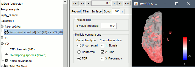
• The statistical result can be displayed similarly to the source files, and you can edit the statistical threshold in the Stat tab. Red values indicate that the power in the alpha band is significantly higher in condition YF (eyes closed). As expected, that parieto-occipital regions appear clearly in this contrast.
  
  

Volume scouts

Some subcortical structures are modeled as volume source structures (for instance here, the thalamus and the amygdala). It is not possible to display scouts time series for these structures from the "Source model" or "Structures" atlases. It is necessary to create a new atlas, specific to volume scouts. Volume scouts are described in the tutorial Volume source estimation. The only difference here is that you will be able to create them from the grid of points you see in the 3D figures (instead of the MRI slices).

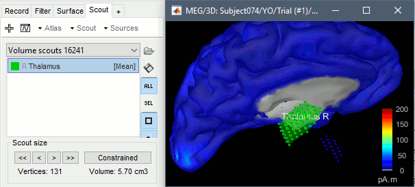
• Double-click on one of the source files (not averaged in time) to open it. From the Surface tab, configure it so you see the grid of points corresponding to the right thalamus (make the surface 100% transparent, or hide the right hemisphere).

• In the Scout tab, menu Atlas > New atlas > Volume scouts.
  
  

• Click on the button [Create scout], click on one of the points of the right thalamus. Then grow it until it includes all the sources in the structure. Rename it to "Thalamus R".
  
  

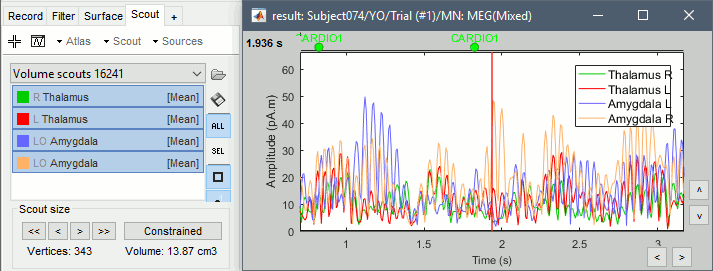
• Repeat these steps for all the regions you are interested in and display the scouts time series.
  
  

References

Attal Y, Bhattacharjee M, Yelnik J, Cottereau B, Lefèvre J, Okada Y, Bardinet E, Chupin M, Baillet S (2009)
Modelling and detecting deep brain activity with MEG and EEG
IRBM, 30(3):133-138

Attal Y, Schwartz D (2013)
Assessment of Subcortical Source Localization Using Deep Brain Activity Imaging Model with Minimum Norm Operators: A MEG Study
PLOS ONE, 8(3):e59856

Dumas T, Dubal S, Attal Y, Chupin M, Jouvent R (2013)
MEG Evidence for Dynamic Amygdala Modulations by Gaze and Facial Emotions
PLOS ONE, 8(9): e74145

Additional documentation

• Forum: https://neuroimage.usc.edu/forums/t/gain-matrix-computation-including-subcortical-structures/30818

Scripting

The following script from the Brainstorm distribution reproduces the analysis presented in this tutorial page: brainstorm3/toolbox/script/tutorial_dba.m