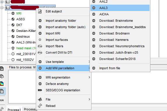
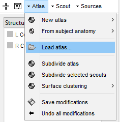
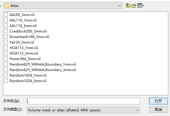
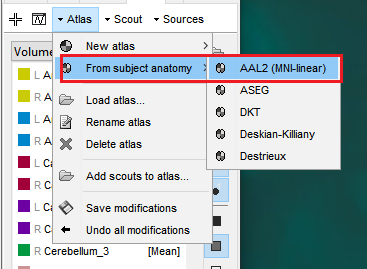
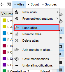
I am sorry to bother you. I am currently working on brain network connectivity based on the AAL atlas and have discovered two methods to apply it: one is to directly import it into the anatomical folder of the subject (Figure1), and the other is to load the atlas, as illustrated in Figures 2 and 3. Could you kindly explain the differences between these two approaches?
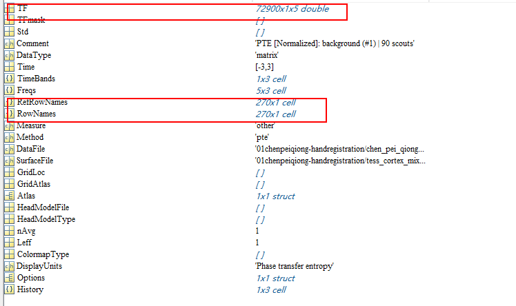
Additionally, when I calculate the PTE brain network using 90 brain regions, the resulting network size is 270270=72,900, as shown in Figure 4. Could you please guide me on how to reduce this to a 9090 connectivity matrix?
On the Scout tab, the Atlas is a scout ** atlas**, this is to say a collection of surface (or volume) scouts, where each scout is a collection of vertices from the source space (cortical surface or brain volume).
It will depend on your research question, some Scout functions would emphasize scout tendencies, where other will highlight only the high connectivity metrics. Also consider that the Scout function can be applied before or after. Check this link for further information on the different ways to compute connectivity using Scouts:
Thank you for your reply. Your answer has been very helpful.
However, I am still a bit confused: after loading the AAL atlas in the Anatomy view, I can import the AAL atlas into the Scout tab via "From subject anatomy" (Figure 1). Alternatively, I can directly use "Load atlas" in the Scout tab to import the atlas (Figures 2-3). Is there a difference between these two methods? Looking forward to your response.
That is a interesting question. I see that you are working with volume source space. Under certain circumstances these two methods are almost the same. Let me expand.
On the first approach, "From subject anatomy", there is a MRI volume already in the subject space (either from the MRI segmentation, or the anatomical parcellation was imported from the MNI space), then for each vertex in the volume source space, a label is assigned according to label of the anatomical parcellation in the subject space.
For the second approach, "Load atlas", as you can see there are several options to import. In your image, you are importing it as dilated, MNI space. Thus, for each vertex in the volume source space, a label is assigned according to its MNI coordinates, and the label of the anatomical parcellation in that location. With the dilated option, each ROI in the anatomical parcellation is inflated before, see the full explanation in here: