Granger causality
Authors: Hossein Shahabi and Raymundo Cassani
This tutorial extends the information provided in the connectivity tutorial regarding the formulation of time- and frequency-domain Granger causality. Moreover, an numeric example based on simulated signals is provided to verify the results obtained with GC in time and frequency domain.
Contents
Mathematical background
Wiener-Granger causality, better know as Granger causality (GC) is a method of functional connectivity, while conceptually developed by Norbert Wiener in 1956, it was implemented in terms of linear autoregressive modelling by Clive Granger in the 1960s (Granger, 1969), but later refined by John Geweke in the form that is used today (Geweke, 1984). Granger causality was originally formulated in economics, but has caught the attention of the neuroscience community in recent years. Before this, neuroscience traditionally relied on lesions and applying stimuli on a part of the nervous system to study it’s effect on another part. However, Granger causality made it possible to estimate the statistical influence without requiring direct intervention (Bressler and Seth, 2011).
By definition, Granger causality is a measure of linear dependence, which tests whether the variance of error for a linear autoregressive model estimation (AR model) of a signal  can be reduced when adding a linear model estimation of a second signal
  . If this is true, signal
  has a Granger causal effect on the first signal
  , i.e., independent information of the past of
  improves the prediction of
  above and beyond the information contained in the past of
  alone. The term independent is emphasized because it creates some interesting properties for GC, such as that it is invariant under rescaling of the signals, as well as the addition of a multiple of
  to
to  . The measure of Granger Causality is nonnegative, and zero when there is no Granger causality (Geweke, 1984).
The main advantage of Granger causality is that it is an directed measure, in that it can dissociate between  versus
  . It is important to note however that though the directionality of Granger causality is a step closer towards measuring effective connectivity compared to non-directed measures, it should still not be confused with “true causality”. Effective connectivity estimates the effective mechanism generating the observed data (model based approach), whereas GC is a measure of causal effect based on prediction, i.e., how well the model is improved when taking variables into account that are interacting (data-driven approach) (Barrett and Barnett, 2013).
The difference with causality is best illustrated when there are more variables interacting in a system than those taken into account in the model. For example:
A variable  is causing both
  and
and  , but with a smaller delay for
  than for
In its simplest (unconditional) form, Granger causality measure between The spurious causalities like in the example above, may be removed by using the IMAGE
Even though GC has been extended for nonlinear, multivariate and time-varying conditions, in this tutorial we will stick to the basic case, which is a linear, bivariate and stationary model defined in both the time and spectral domain. In the time domain this can be represented in the following way.
If Where Which is 0 for
TODO: RC
An important improvement by Geweke was to show that under fairly general conditions,
If the two AR models in time domain are specified as: In each equation the reduced model can be defined when each signal is an AR model of only its own past, with error terms where Rewriting this as Where Finally, assuming independence of the signals Note that the ability to reformulate the equations in spectral domain also makes it very easy to generalize to a multivariate GC. That is why all multivariate measures of GC are defined in spectral domain. Alternative measures derived from these multivariate autoregressive estimates are Partial Directed Coherence (PDC) and Directed Transfer Function (DTF).
TODO: RC
In the next sections we present a hands-on example with simulated signals where Granger causality (in time and frequency domain) can be used. Since the GC method is based on AR modelling of signals, the simulated signals are generated with a AR model, thus providing a fair ground truth to validate the GC results.
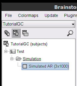
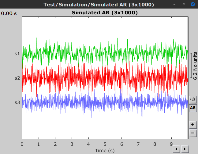
In this example, we generate a dataset for a 3-variate AR model (example 2 in the study of (Baccala and Sameshima, 2001)). These observed time series are assumed to be generated by the equations: Where To do simulate this in Brainstorm, we use the following steps: Select the menu File > Create new protocol > "TutorialGC" and select the options: In the Select the process Which is a 10 second simulation with 100Hz sampling rate. The process will give you a data file presented in Brainstorm as: When displaying the data as time-series:
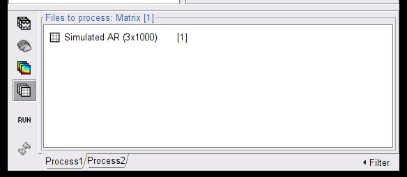
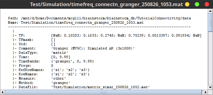
To compute Granger causality, place the simulated data in the Click on The connectivity profile calculated is saved in the file You also have the option of showing the results as a graph with right-click on the Granger file then (figure 7)
The output of the
The Where On a similar note, the As mentioned in the introduction, the current model is based on the assumption of stationarity. Therefore it is important to first check if the time series we are using are stationary with statistical tests such as the KPSS test or the Dickey-Fuller (unit root) test. If the data is shown to be non-stationary, certain techniques can still render it stationary (depending on the type of non-stationarity). A common approach is to difference the data to eliminate any trends in the time series (i.e., $x_t^{'}=x_{t}-x_{t-1}$). This can be done several times if necessary. A problem with this is that it could potentially change the interpretation of any resulting GC, specifically in the frequency domain where differencing acts as a high filter. Other commonly used methods are smoothing or filtering the data, but in the end if there are causal relation that vary over time these technique will make it impossible to find those. An alternative approach could be to divide the data into time-series that are (sufficiently) locally stationary, and apply the GC per time window. This method makes is possible to study changes in connectivity over time, but it is of course not without its own problems, the most important of which is the choice of the
To estimate GC in frequency domain, drag the the simulated signals to the Click on As with the temporal GC, right-click on the SpGranger file, and select
With respect to (temporal) GC, spectral GC presents two extra parameters:
The output of the
Granger CW. Geweke JF. Bressler SL, Seth AK. Baccalá LA, Sameshima K. Barnett L, Seth AK.
Connectivity matrix storage:http://neuroimage.usc.edu/forums/showthread.php?1796  and
and  would show a non-zero GC for
  -->
-->  , even though
  is not truly causing
  (Bressler and Seth, 2011).
 and
and  considering
  in the modelling, this is to say
  -->
-->  |
| (where '|' means 'conditioned on') would be close to zero. (Barnett and Seth 2014).
 GC in time domain
Unconditional GC
 represents a signal that can be modelled using a linear AR model in the following two ways:
 ![\begin{eqnarray*}
x(t) & = & \sum_{k=1}^{p} [A_{k}x(t-k)] +e_1 \\
x(t) & = & \sum_{k=1}^{p} [A_{k}x(t-k)+B_{k}y(t-k)] +e_2
\end{eqnarray*} \begin{eqnarray*}
x(t) & = & \sum_{k=1}^{p} [A_{k}x(t-k)] +e_1 \\
x(t) & = & \sum_{k=1}^{p} [A_{k}x(t-k)+B_{k}y(t-k)] +e_2
\end{eqnarray*}](/brainstorm/GrangerCausality?action=AttachFile&do=get&target=latex_ff96bd67f304dfa4455accf112cb1620facee597_p1.png)
 is the
  uses the past (and present) of only itself whereas the second includes the past (and present) of a second signal
  . Note that when only past measures of signals are taken into account (
 ), the model ignores simultaneous connectivity, which makes it less susceptible to volume conduction (Cohen, 2014). Then, according to the original formulation of GC, the measure of GC from
  to
to  is defined as:
 and a non-negative value for
  . Note that
  always holds, as the model can only improve when adding new information.
 Conditional GC
GC in frequency domain
 can be decomposed by frequency.
 Unconditional spectral GC
![\begin{eqnarray*}
x(t) &=\sum_{k=1}^{p} [A_{k_{xx}}x(t-k) + A_{k_{xy}}y(t-k)] +\sigma_{xy} \\
y(t) &=\sum_{k=1}^{p} [A_{k_{yy}}y(t-k) + A_{k_{yx}}y(t-k)] +\sigma_{yx}
\end{eqnarray*} \begin{eqnarray*}
x(t) &=\sum_{k=1}^{p} [A_{k_{xx}}x(t-k) + A_{k_{xy}}y(t-k)] +\sigma_{xy} \\
y(t) &=\sum_{k=1}^{p} [A_{k_{yy}}y(t-k) + A_{k_{yx}}y(t-k)] +\sigma_{yx}
\end{eqnarray*}](/brainstorm/GrangerCausality?action=AttachFile&do=get&target=latex_7053c1d2e3c64970fd2e3c0b13042ca58f9fcdc7_p1.png)
 and
and  . Then we can defined the variance-covariance matrix of the whole system as:
 ![\begin{eqnarray*}
\Sigma =
\left[\begin{array}{cc}
\Sigma_{xx} & \Sigma_{xy} \\
\Sigma_{yx} & \Sigma_{yy}
\end{array}\right] \\
\end{eqnarray*} \begin{eqnarray*}
\Sigma =
\left[\begin{array}{cc}
\Sigma_{xx} & \Sigma_{xy} \\
\Sigma_{yx} & \Sigma_{yy}
\end{array}\right] \\
\end{eqnarray*}](/brainstorm/GrangerCausality?action=AttachFile&do=get&target=latex_9b11baf00d9a911511636a10c2e8757b493a8102_p1.png)
 , etc. Applying the the Fourier transform to these equations, they can be expressed as:

 is the transfer matrix. The spectral matrix is then defined as:
 and
and  , and
, and  , we can define the spectral GC as:
Conditional spectral GC
A few noteworthy practical issues about GC
Temporal resolution: the high time resolution offered by MEG, EEG, and intracranial EEG allows for a very powerful application of GC and also offers the important advantage of spectral analysis.  ) where
  represents the number of variables). Since each connection pair results in two values, there will also be a large number of statistical comparisons that need to be controlled for. When performing GC in the spectral domain, this number increases even more as statistical tests have to be performed per frequency. Therefore it is usually recommended to select a limited number of ROIs or electrodes based on some hypothesis found in previous literature, or on some initial processing with a more simple and less computationally heavy measure of connectivity.
 Simulate signals

 are zero-mean uncorrelated white processes with identical variances. Since the model order in this example is one, we can rewrite the equations in matrix form as such:
Process1 tab, leave the file list empty and click on the button [Run] ( ![]() ) to open the Pipeline editor.
) to open the Pipeline editor. % Coefficient matrix A:
A1 = [ 0.5 0.3 0.4;
-0.5 0.3 1.0;
0.0 -0.3 -0.2];
A = [A1];
% Intercept b:
b = [0 0 0];
% Noise covariance matrix C:
C = eye(3,3);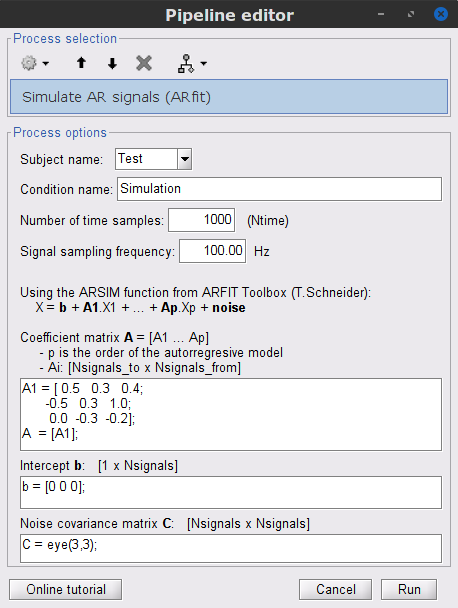
Process options
Subject name: Specify in which subject the simulated file is saved. Bivariate (temporal) Granger Causality NxN
Process1 tab.
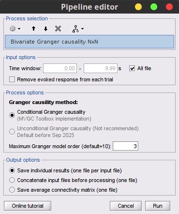
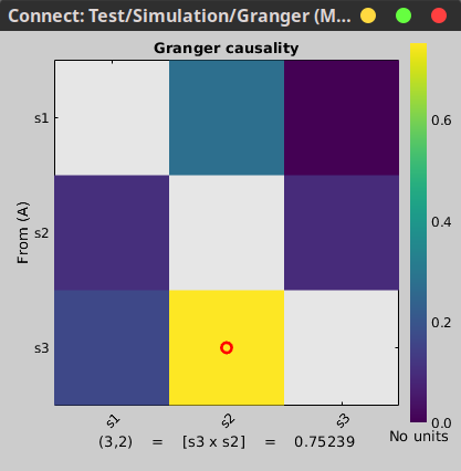
In this image, an asymmetrical matrix of GC estimates is shown, with non-negative values. Note that this map is not a multivariate analysis of our multivariate system, but instead a 3-by-3 bivariate analysis. It is known that bivariate connectivity measures to estimate the correct pattern of propagation in a multivariate system can be problematic, nevertheless the results still show a pretty good estimation of connectivity, as can be seen in the strong propagation of activity going from signal 3 to signal 2, as is the case in the originally described model. The next strong connections are from signal 1 to signal 2, and from signal 3 to signal 1. Note that connections from signal 2 to signal 1, and from signal 2 to signal 3 show similar values, as they have the same coefficient value in the simulation model though with negative signs. Note that the relative strengths of connectivity in the results are reserved, but the value itself is a ratio of the residual errors of the full and reduced model as described in the introduction, and should not be confused with the actual coefficient values. Process options
Time window: Segment of the signal used for the connectivity analysis. Check All file. On the hard drive
Recommendations

 is the noise covariance matrix,
  model order,
  number of variables, and
  is the number of data samples.
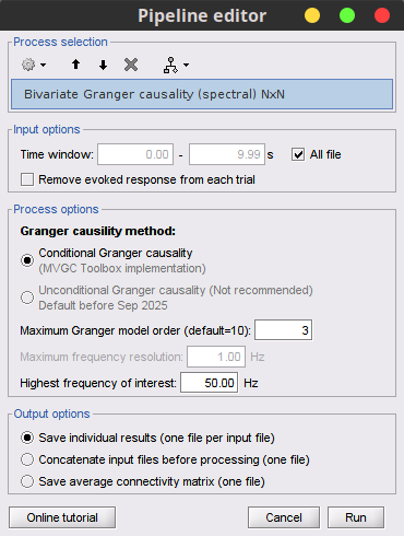
 Bivariate spectral Granger causality NxN
Process1 tab.

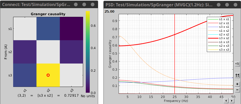
Where the first variable in the legend refers to the sender and the second to the receiver of information. As we can see from the figure the large coupling strength from signal 2 to signal 3 is highest in higher frequency ranges. You can select your desired connectivity pair, and then press enter to view it in a separate window. Process options
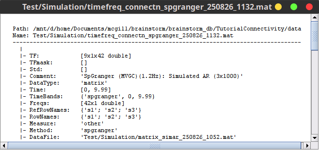
Maximum frequency resolution: Width of frequency bins in PSD estimation. A large number of steps (high resolution) will increase the number of statistical comparisons. Note that the frequency resolution has to be less than half the highest frequency of interest. On the hard drive
Additional documentation
Articles
Investigating causal relations by econometric models and cross-spectral methods.
Econometrica: journal of the Econometric Society. 1969;424–38.
Measures of conditional linear dependence and feedback between time series.
Journal of the American Statistical Association. 1984;79(388):907–15.
Wiener–Granger causality: a well established methodology.
Neuroimage. 2011 Sep 15;58(2):323-9.
Partial directed coherence: a new concept in neural structure determination.
Biol Cybern. 2001 May 11;84(6):463–74.
The MVGC multivariate Granger causality toolbox: A new approach to Granger-causal inference.
Journal of Neuroscience Methods. 2014. Forum discussions
