Corticomuscular coherence (CTF MEG)

Authors: Raymundo Cassani, Francois Tadel, Sylvain Baillet.

Corticomuscular coherence measures the degree of similarity between electrophysiological signals (MEG, EEG, ECoG sensor traces or source time series, especially over the contralateral motor cortex) and the EMG signals recorded from muscle activity during voluntary movements. Cortical-muscular signals similarities are conceived as due mainly to the descending communication along corticospinal pathways between primary motor cortex (M1) and the muscles attached to the moving limb(s). For consistency purposes, the present tutorial replicates, with Brainstorm tools, the processing pipeline "Analysis of corticomuscular coherence" of the FieldTrip toolbox.

Dataset description

The dataset is identical to that of the FieldTrip tutorial: Analysis of corticomuscular coherence:

• One participant,
• MEG recordings: 151-channel CTF MEG system,
• Bipolar EMG recordings: from left and right extensor carpi radialis longus muscles,
• EOG recordings: used for detection and attenuation of ocular artifacts,
• MRI: 1.5T Siemens system,
• Task: The participant lifted their hand and exerted a constant force against a lever for about 10 seconds. The force was monitored by strain gauges on the lever. The participant performed two blocks of 25 trials using either their left or right hand.
• Here we describe relevant Brainstorm tools via the analysis of the left-wrist trials. We encourage the reader to practice further by replicating the same pipeline using right-wrist trials!

Corticomuscular coherence:

• Coherence measures the linear relationship between two signals in the frequency domain.

• Previous studies (Conway et al., 1995, Kilner et al., 2000) have reported corticomuscular coherence effects in the 15–30 Hz range during maintained voluntary contractions.

• TODO: IMAGE OF EXPERIMENT, SIGNALS and COHERENCE

Download and installation

Pre-requisites

• Please make sure you have completed the get-started tutorials, prior to going through the present tutorial.

• Have a working copy of Brainstorm installed on your computer.

• Install the CAT12 Brainstorm plugin, to perform MRI segmentation from the Brainstorm dashboard.

Download the dataset

• Download SubjectCMC.zip from the FieldTrip download page:
  https://download.fieldtriptoolbox.org/tutorial/SubjectCMC.zip

• Unzip the downloaded archive file in a folder outside the Brainstorm database or app folders (for instance, directly on your desktop).

Brainstorm

• Launch Brainstorm (via the Matlab command line or the Matlab-free stand-alone version of Brainstorm).

• Select from the menu File > Create new protocol. Name the new protocol TutorialCMC and select the options:
  No, use individual anatomy,
  No, use one channel file per acquisition run.

Importing anatomy

• Right-click on the newly created TutorialCMC node > New subject > Subject01.
  Keep the default options defined for the study (aka "protocol" in Brainstorm's vernacular).

• Switch to the Anatomy view of the protocol ().

• Right-click on the Subject01 > Import MRI:

  • Select the file format: All MRI files (subject space)

  • Select the file: SubjectCMC/SubjectCMC.mri

• This step will launch Brainstorm's MRI viewer, where coronal, sagittal and axial cross-sections of the MRI volume are displayed. note that three anatomical fiducials (left and right pre-auricular points (LPA and RPA), and nasion (NAS)) are automatically identified. These fiducials are located near the left/right ears and just above the nose, respectively. Click on Save.
  
  

• In all typical Brainstorm workflows from this tutorial handbook, we recommend processing the MRI volume at this stage, before importing the functional (MEG/EEG) data. However, we will proceed differently, for consistency with the original FieldTrip pipeline, and readily obtain sensor-level coherence results. We will proceed with MRI segmentation below, before performing source-level analyses.

• We still need to verify the proper geometric registration (alignment) of MRI with MEG. We will therefore now extract the scalp surface from the MRI volume.

• Right-click on the MRI () > MRI segmentation > Generate head surface.
  
  

• Double-click on the newly created surface to display the scalp in 3-D.
  
  

MEG and EMG recordings

Link the recordings

• Switch now to the Functional data view of your database contents ().

• Right-click on Subject01 > Review raw file:

  • Select the appropriate MEG file format: MEG/EEG: CTF(*.ds; *.meg4; *.res4)

  • Select the data file: SubjectCMC.ds

• A new folder SubjectCMC is created in the Brainstorm database explorer. Note the "RAW" tag over the icon of the folder (), indicating that the MEG files contain unprocessed, continuous data. This folder includes:

• CTF channels (191) is a file with all channel information, including channel types (MEG, EMG, etc.), names, 3-D locations, etc. The total number of channels available (MEG, EMG, EOG etc.) is indicated between parentheses.

• Link to raw file is a link to the original data file. Brainstorm reads all the relevant metadata from the original dataset and saves them into this symbolic node of the data tree (e.g., sampling rate, number of time samples, event markers). As seen elsewhere in the tutorial handbook, Brainstorm does not create copies by default of (potentially large) unprocessed data files (more information).

• 
  

MEG-MRI coregistration

• This registration step is to align the MEG coordinate system with the participant's anatomy from MRI (more info). Here we will use only the three anatomical landmarks stored in the MRI volume and specific at the moment of MEG data collection. From the FieldTrip tutorial:
  "To measure the head position with respect to the sensors, three coils were placed at anatomical landmarks of the head (nasion, left and right ear canal). [...] During the MRI scan, ear molds containing small containers filled with vitamin E marked the same landmarks. This allows us, together with the anatomical landmarks, to align source estimates of the MEG with the MRI."

• To visually appreciate the correctness of the registration, right-click on the CTF channels node > MRI registration > Check. This opens a 3-D figure showing the inner surface of the MEG helmet (in yellow), the head surface, the fiducial points and the axes of the subject coordinate system (SCS).
  
  

Reviewing

• Right-click on the Link to raw file > Switch epoched/continuous to convert how the data i stored in the file to a continuous reviewing format, a technical detail proper to CTF file formatting.

• Right-click on the Link to raw file > MEG > Display time series (or double-click on its icon). This will display data time series and enable the Time panel and the Record tab in the main Brainstorm window (see specific features in "explore data time series").

• Right-click on the Link to raw file > EMG > Display time series.

• 

Event markers

The colored dots at the top of the figure, above the data time series, indicate event markers (or triggers) saved along with MEG data. The actual onsets of the left- and right-wrist trials are not displayed yet: they are saved in an auxiliary channel of the raw data named Stim. To add these markers to the display, follow this procedure:

• With the time series figure still open, go to the Record tab and select File > Read events from channel. Event channels = Stim, select Value, Reject events shorter than 12 samples. Click Run.

• 

• The rejection of short events is nececessary in this dataset, because transitions between values in the Stim channel may span over several time samples. Otherwise, and for example, an event U1 would be created at 121.76s because the transition from the event U1025 back to zero features two unwanted values at the end of the event. The rejection criteria is set to 12 time samples (10ms), because the duration of all the relevant triggers is longer than 15ms. This value is proper to each dataset, so make sure you verify trigger detections from your own dataset.
  
  

• New event markers are created and now shown in the Events section of the tab, along with previous event categories. In this tutorial, we will only use events U1 through U25, which correspond to the beginning of each of the 25 left-wrist trials of 10 seconds. Following FieldTrip's tutorial, let's reject trial #7, event U7.

• Delete all unused events: Select all the events except U1-U6 and U8-25 (Ctrl+click / Shift+click), then menu Events > Delete group (or press the Delete key).

• Merge events: Select all the event groups, then select from the menu Events > Merge group > "Left". A new event category called "Left" now indicate the onsets of 24 trials of left-wrist movements.
  
  

Pre-processing

Power line artifacts

• In the Process1 box: Drag and drop the Link to raw file.

• Run process Frequency > Power spectrum density (Welch):
  

  • Time window: 0-330 s

  • Window length: 10 s

  • Overlap: 50%

  • Sensor types: MEG, EMG

• 

• Double-click on the new PSD file to visualize the power spectrum density of the data.
  

• 

• The PSD plot shows two groups of sensors: EMG (highlighted in red above) and the MEG spectra below (black lines). Peaks at 50Hz and harmonics (100, 150, 200Hz and above) indicate the European power line frequency and are clearly visible. We will now use notch filters to attenuate power line contaminants at 50, 100 and 150 Hz.

• In the Process1 box: Drag and drop the Raw | clean node.

• Run the process Pre-processing > Notch filter with:
  

  • Check Process the entire file at once

  • Sensor types: MEG, EMG

  • Frequencies to remove (Hz): 50, 100, 150

• 

• In case you get a memory error message:
  These MEG recordings have been saved before applying the CTF 3rd-order gradient compensation, for noise reduction. The compensation weights are therefore applied on the fly when Brainstorm reads data from the file. However, this requires reading all the channels at once. By default, the frequency filter are optimized to process channel data sequentially, which is incompatible with applying the CTF compensation on the fly. This setting can be overridden with the option Process the entire file at once, which requires loading the entire file in memory at once, which may crash teh process depending on your computing resources (typically if your computer's RAM < 8GB). If this happens: run the process Artifacts > Apply SSP & CTF compensation on the file first, then rune the notch filter process without the option "Process the entire file at once" (more information).

• A new folder named SubjectCMC_clean_notch is created. Obtain the PSD of these data to appreciate the effect of the notch filters. As above, please remember to indicate a Time window restricted from 0 to 330 s in the options of the PSD process.
  
  

• 

EMG: Filter and rectify

Two typical pre-processing steps for EMG consist in high-pass filtering and rectifying.

• In the Process1 box: drag and drop the Raw | notch(50Hz 100Hz 150Hz) node.

• Add the process Pre-process > Band-pass filter

  • Sensor types = EMG

  • Lower cutoff frequency = 10 Hz

  • Upper cutoff frequency = 0 Hz

• Add the process Pre-process > Absolute values

  • Sensor types = EMG

• Run the pipeline

• 

• Delete intermediate files that won't be needed anymore: Select folders SubjectCMC_notch and SubjectCMC_notch_high, then press the Delete key (or right-click > File > Delete).
  
  

MEG: Blink SSP and bad segments

Stereotypical artifacts such eye blinks and heartbeats can be identified from their respective characteristic spatial distributions. Their contamination of MEG signals can then be attenuated specifically using Signal-Space Projections (SSPs). For more details, consult the specific tutorial sections about the detection and removal of artifacts with SSP. The present tutorial dataset features an EOG channel but no ECG. We will therefore only remove artifacts caused by eye blinks.

Blink correction with SSP

• Right-click on the pre-processed file > MEG > Display time series and EOG > Display time series.

• In the Record tab: Artifacts > Detect eye blinks, and use the parameters:

  • Channel name= EOG

  • Time window = 0 - 330 s

  • Event name = blink

• 

• Three categories of blink events are created. Review the traces of the EOG channels around a few of these events to ascertain they are related to eye blinks. In the present case, we note that the blink group contains genuine eye blinks, and that groups blink2 and blink3 capture saccades.

• 

• To remove blink artifacts with SSP, go to Artifacts > SSP: Eye blinks:

  • Event name=blink

  • Sensors=MEG

• 

• Display the time series and topographies of the first two SSP components identified. In the present case, only the first SSP component can be clearly related to blinks: the percentage of variance explained is substantially higher than the other compoments', the spatial topography of the component is also typical of eye blinks, and the corresponding time series is similar to the EOG signal around blinks. Select only component #1 for removal.

• 

• Close all visualization figures by clicking on the large × at the top-right of the main Brainstorm window.

Detection of "bad" data segments

Here we will use the automatic detection of artifacts to identify data segments contaminated by e.g., large eye and head movements, or muscle contractions.

• Display the MEG and EOG time series. In the Record tab, select Artifacts > Detect other artifacts and enter the following parameters:

  • Time window = 0 - 330 s

  • Sensor types=MEG

  • Sensitivity=3

  • Check both frequency bands 1-7 Hz and 40-240 Hz

• 

• You are encouraged to review all the segments marked using this procedure. With the present data, all marked segments do contain clear artifacts.

• Select the 1-7Hz and 40-240Hz event groups and select Events > Mark group as bad. Alternatively, you can add the prefix bad_ to the event names. Brainstorm will automatically discard these data segments from further processing.

• 

• Close all visualization windows and reply "Yes" to the save the modifications query.

Epoching

We are now finished with the pre-processing of EMG and MEG recordings. We will now extract and import specific data segments of interest into the Brainstorm database for further derivations. As mentioned previously, we will focus on the Left category of events (left-wrist movements). For consistency with the FieldTrip tutorial, we will analyze 8s of recordings following each movement (from the original 10s around each trial), and split them in 1-s epochs. For each 1-s epoch, the DC offset will be also removed from each MEG channel. And finally, we will uniform the time vector for all 1-s epochs. This last steps is needed as the time vector of each 1-s vector is with respect to the event that was used to import the 8-s trial.

• In the Process1 box: Drag-and-drop the pre-processed file.

• Select the process Import > Import recordings > Import MEG/EEG: Events:

  • Subject name = Subject01

  • Folder name = empty

  • Event names = Left

  • Time window = 0 - 330 s

  • Epoch time = 0 - 8000 ms

  • Split recordings in time blocks = 1 s

  • Uncheck Create a separate folder for each event type

  • Check Ignore shorter epochs

  • Check Use CTF compensation

  • Check Use SSP/ICA projectors

• Add the process Pre-process > Remove DC offset:

  • Baseline = All file

  • Sensor types = MEG

  • Check Overwrite input files

• Add the process Standardize > Uniform epoch time:

  • Interpolation method = spline

  • Check Overwrite input files

• Run the pipeline

• A new folder SubjectCMC_notch_high_abs without the 'raw' indication is now created, which includes 192 individual epochs (24 trials x 8 1-s epochs each). The epochs that overlap with a "bad" event are also marked as bad, as shown with an exclamation mark in a red circle (). These bad epochs will be automatically ignored by the Process1 and Process2 tabs, and from all further processing.

• 

Comparison with FieldTrip

The figures below show the EMG and MRC21 channels (a MEG sensor over the left motor-cortex) from the epoch #1.1, in Brainstorm (left), and from the FieldTrip tutorial (right).

Coherence: EMG x MEG

Let's compute the magnitude-squared coherence (MSC) between the left EMG and the MEG channels.

• In the Process1 box, drag and drop the Left (192 files) trial group.

• 

• Select the process Connectivity > Coherence 1xN [2023]:

  • Time window = Check All file

  • Source channel = EMGlft

  • Sensor types = MEG

  • Do not check Include bad channels

  • Select Magnitude squared coherence as Connectivity metric

  • Select Fourier transform as Time-freq decomposition method

  • Click in the [Edit] button to set the parameters of the Fourier transform:

    • Select Matlab's FFT defaults as Frequency definition

    • FT window length = 0.5 s

    • FT window overlap = 50%

    • Highest frequency of interest = 80 Hz

  • Time resolution = None

  • Estimate & save = across combined files/epochs

  More details on the Coherence process can be found in the Connectivity Tutorial.

• Add the process File > Add tag with the following parameters:

  • Tag to add = MEG sensors

  • Select Add to file name

• Run the pipeline:

• Double-click on the resulting data node MSCoh-stft: EMGlft (185 files) | MEG sensors to display the MSC spectra. Click on the maximum peak in the 15 to 20 Hz range, and press Enter to display the spectrum from the selected sensor in a new window. This spectrum is that of channel MRC21, and shows a prominent peak at 17.58 Hz. Use the frequency slider (under the Time panel) to explore the MSC output across frequencies.

• Right-click on the spectrum and select 2D Sensor cap for a topographical representation of the magnitude of the coherence results across the sensor array. You may also use the shortcut Ctrl-T. The sensor locations can be displayed with a right-click and by selecting Channels > Display sensors from the contextual menu (shortcut Ctrl-E).

• 

• We can now average the magnitude of the MSC across the beta band (15-20 Hz).
  In the Process1 box, select the new mscohere file.

• Run process Frequency > Group in time or frequency bands:

  • Select Group by frequency bands

  • Type cmc_band / 15, 20 / mean in the text box.

• 

• The resulting MSCoh-stft:...|tfbands node contains one MSC value for each sensor (the MSC average in the 15-20 Hz band). Right-click on the file to display the 2D or 3D topography of the MSC beta-band measure.
  
  

• Higher MSC values the EMG signal and MEG sensor signals map over the contralateral set of central sensors in the beta band. Sensor-level connectivity can be ambiguous to interpret anaotmically though. We will now map the magnitude of EMG-coherence across the brain (MEG sources).

Source estimation

MRI segmentation

We first need to extract the cortical surface from the T1 MRI volume we imported at the beginning of this tutorial. CAT12 is a Brainstorm pluing that will perform this task in 30-60min.

• Switch back to the Anatomy view of the protocol ().

• Right-click on the MRI () > MRI segmentation > CAT12:

  • Number of vertices: 15000

  • Anatomical parcellations: Yes

  • Cortical maps: No

• 

• Keep the low-resolution central surface selected as the default cortex (central_15002V). This surface is the primary output of CAT12, and is shown half-way between the pial envelope and the grey-white interface (more information). The head surface was recomputed during the process and duplicates the previous surface obtained above: you can either delete one of the head surfaces or ignore this point for now.

• For quality control, double-click on the head and central_15002V surfaces to visualize them in 3D.
  
  

Head models

We will perform source modeling using a distributed model approach for two different source spaces: the cortex surface and the entire MRI volume. Forward models are called head models in Brainstorm. They account for how neural electrical currents produce magnetic fields captured by sensors outside the head, considering head tissues electromagnetic properties and geometry, independently of actual empirical measurements (more information). A distinct head model is required for the cortex surface and head volume source spaces.

Cortical surface

• Go back to the Functional data view of the database.

• Right-click on the channel file of the imported epoch folder > Compute head model.

  • Comment = Overlapping spheres (surface)

  • Source space = Cortex surface

  • Forward model = MEG Overlapping spheres.

• 

Whole-head volume

• Right-click on the channel file again > Compute head model.

  • Comment = Overlapping spheres (volume)

  • Source space = MRI volume

  • Forward model = Overlapping spheres.

  • Select Regular grid and Brain

  • Grid resolution = 5 mm

• 

• The Overlapping spheres (volume) head model is now added to the database explorer. The green color of the name indicates this is the default head model for the current folder: you can decide to use another head model available by double clicking on its name.

• 

Noise covariance

The recommendation for MEG source imaging is to extract basic noise statistics from empty-room recordings. When not available, as here, resting-state data can be used as proxies for MEG noise covariance. We will use a segment of the MEG recordings, away from the task and major artifacts: 18s-29s.

• Right-click on the clean continuous file > Noise covariance > Compute from recordings.
  
  

• Right-click on the Noise covariance () > Copy to other folders.
  
  

Inverse models

We will now compute three inverse models, with different source spaces: cortex surface with constrained dipole orientations (normal to the cortex), cortex surface with unconstrained orientation, and MRI volume (more information).

Cortical surface

• Right-click on Overlapping spheres (surface) > Compute sources:

  • Minimum norm imaging

  • Current density map

  • Constrained: Normal to the cortex

  • Comment = MN: MEG (surface)

• Repeat the previous step, but this time select Unconstrained in the Dipole orientations field.

Whole-head volume

• Right-click on the Overlapping spheres (volume) > Compute sources:

  • Current density map

  • Unconstrained

  • Comment = MN: MEG (volume)

• 

• Three imaging kernels () are now available in the database explorer. Note that each trial is associated with three source links (). The concept of imaging kernels is explained in Brainstorm's main tutorial on source mapping.

• 

Coherence: EMG x Sources

We can now compute the coherence between the EMG signal and all brain source time series, for each of the source models considered. This computation varies if we are using constrained or unconstrained sources.

Method for constrained sources

For cortical and orientation-constrained sources, each vertex in the source grid is associated with 1 time series. As such, when coherence is computed with the EMG signal (also consisting of one time series), this result is 1 coherence spectrum per vertex. In other words, for each frequency bin, we obtain one coherence brain map.

Let's compute coherence between the EMG sensor and the sources from the cortical surface/constrained model.

• To select the source maps to include in the coherence estimation, click on the Search Database button (), and select New search. Set the parameters as shown below, and click on Search.

• 

• This creates a new tab in the database explorer, showing only the files that match the search criteria.

• 

• Click the Process2 tab at the bottom of the main Brainstorm window.

  • Files A: Drag-and-drop the Left (192 files) group, select Process recordings ().

  • Files B: Drag-and-drop the Left (192 files) group, select Process sources ().

  • Objective: Extract from the same files both the EMG recordings (Files A) and the sources time series (Files B), then compute the coherence measure between these two categories of time series. Note that the blue labels over the file lists indicate that there are 185 "good" files (7 bad epochs).

• 

• Select the process Connectivity > Coherence AxB [2023]:

  • Time window = All file

  • Source channel (A) = EMGlft

  • Uncheck Use scouts (B)

  • Ignore the Scout function options as we are not using scouts

  • Select Magnitude squared coherence as Connectivity metric

  • Select Fourier transform as Time-freq decomposition method

  • Click in the [Edit] button to set the parameters of the Fourier transform:

    • Select Matlab's FFT defaults as Frequency definition

    • FT window length = 0.5 s

    • FT window overlap = 50%

    • Highest frequency of interest = 80 Hz

  • Time resolution = None

  • Estimate & save = across combined files/epochs

• Add the process File > Add tag:

  • Tag to add = (surface)(Constr)

  • Select Add to file name

• Run the pipeline

  The parameters Flatten unconstrained source orientations and PCA options do not have any impact on constrained sources, as these already consist on one time series per source location.

Double-click on the 1xN connectivity file for the two (surface) source spaces (constrained and unconstrained source orientations) to visualize the cortical maps. See main tutorial Display: Cortex surface for all available options. Pick the cortical location and frequency with the highest coherence value.

Method for unconstrained sources

In the case of orientation-unconstrained (either surface or volume) sources, each vertex (source location) is associated with 3 time series, each one corresponding to the X, Y and Z directions. Thus, a dimension reduction across directions is needed. In this tutorial the dimension reduction consisted in flattening the unconstrained maps to a single orientation with the PCA method. This results in a source model similar to that with orientation-constrained sources, thus, coherence is then computed as with orientation-constrained (described above).

Let's compute coherence between the EMG sensor and: the sources from the cortical surface/unconstrained and brain volume/unconstrained models.

• Select the sensor and sources files as in the [[|previous section]] for the the source unconstrained model: surface/unconstrained, to have the same files both the EMG recordings (Files A) and the sources time series (Files B), then compute the coherence measure between these two categories of time series:
  

• Select the process Connectivity > Coherence AxB [2023]:

  • Time window = All file

  • Source channel (A) = EMGlft

  • Uncheck Use scouts (B)

  • Check Flatten unconstrained source orientations

  • Click in the [Edit] button of the PCA options:

    • Select across all epochs/files as PCA method

    • PCA time window = All file

    • Check Remove DC offset

    • Baseline = All file

  • Ignore the Scout function options as we are not using scouts

  • Select Magnitude squared coherence as Connectivity metric

  • Select Fourier transform as Time-freq decomposition method

  • Click in the [Edit] button to set the parameters of the Fourier transform:

    • Select Matlab's FFT defaults as Frequency definition

    • FT window length = 0.5 s

    • FT window overlap = 50%

    • Highest frequency of interest = 80 Hz

  • Time resolution = None

  • Estimate & save = across combined files/epochs

• Add the process File > Add tag:

  • Tag to add = (surface)(Unconstr)

  • Select Add to file name

• Run the pipeline

Repeat now using the source files form the brain volume/unconstrained model. Do not forget to update the Tag text to (volume)(Unconstr) in the Add tag process.

• An alternative to address the issue of the dimension reduction across directions when estimating coherence with unconstrained sources is to flatten the results after computing coherence. Coherence is computed between the EMG signal (one time series) and each of the 3 time series (one for each source orientation: x, y and z) associated with each source location, resulting in 3 coherence spectra per source location. Then, these coherence spectra are collapsed (flattened) into a single coherence spectrum by keeping the maximum coherence value across those in the three directions for each frequency bin. The choice of the maximum statistic is empirical: it is not rotation invariant (if the specifications of the NAS/LPA/RPA fiducials change, the x,y,z axes also change, which may influence connectivity measures quantitatively). Nevertheless, our empirical tests showed this option produced smooth and robust (to noise) connectivity estimates.

  

Comparison

• Close the search tab. If the 3 new connectivity files ) are not featured in the database explorer: refresh the database display by pressing [F5] or by clicking again on the selected button "Functional data".
  
  

Double-click on the 1xN connectivity files for the two (surface) source spaces (constrained and unconstrained source orientations) to visualize the cortical maps. See main tutorial Display: Cortex surface for all available options. Pick the cortical location and frequency with the highest coherence value.

• In the Surface tab: Smooth=30%, Amplitude=0%.

• To compare visually different cortex maps, set manually the colormap range (e.g.[0 - 0.07])

• Explore with coherence spectra with the frequency slider

• The highest coherence value is located at 14.65 Hz, in the right primary motor cortex (precentral gyrus). To observe the coherence spectrum at a given location: right-click on the cortex > Source: Power spectrum.
  
  

• The constrained (top) and unconstrained (bottom) orientations coherence maps are qualitatively similar in terms of peak location and frequency. The unconstrained source map appears smoother because of the maximum aggregation across all three current directions at each brain location, as explained below. These maps results are similar to those obtained with the FieldTrip tutorial.

• To obtain the 3D coordinates of the peak coherence location: right-click on the figure > Get coordinates. Then click on the right motor cortex with the crosshair cursor. Let's keep note of these coordinates for later comparision with the whole-head volume results below.
  
  

• Double-click the 1xN connectivity file to display the (volume) source space.

• Set the frequency to 14.65 Hz, and the data transparency to 20% (Surface tab).
• Find the peak in the head volume by navigating in all 3 dimensions, or use the coordinates from the surface results as explained above.

• Right-click on the figure > Anatomical atlas > None. The coherence value under the cursor is then shown on the top-right corner of the figure.
  
  

Coherence: EMG x Scouts

We have now obtained coherence spectra at each of the 15002 brain source locations. This is a very large amount of data to shift through. We therefore recommend to further reduce the dimensionality of the source space by using a surface- or volume-parcellation scheme. In Brainstorm vernacular, this can be achieved via an atlas consisting of scout regions. See the Scout Tutorial for detailed information about atlases and scouts in Brainstorm. To compute scout-wise coherence, it is necessary to specify two parameters to indicate how the data is aggregated in each scout:

1. The scout function (for instance, the mean), and

2. When the scout aggregation procedure if performed, either before or after the coherence computation).

Method for constrained sources

When the scout function is used with constrained sources, the computation of coherence is carried as follows:

• If the scout function is applied before: The scout function (e.g., mean) is applied for all the source time series in the scout; resulting in 1 time series per scout. This scout time series is then used to compute coherence with the reference signal (here, with EMG) resulting in 1 coherence spectrum per scout.

• If the scout function applied after: coherence is first computed between the reference signal (here, EMG) and each source time series in the scout, resulting in N coherence spectra, with N being the number of sources in the scout. Finally the scout function is applied to the resulting coherence spectra for each source within the scout to obtain one coherence spectrum per scout. This is a considerably more greedy option that the "before" option above, as it computes coherence measures between the EMG signal and each of the 15000 elementary source signals. This requires more computing resources; see introduction for an example.

Method for unconstrained sources

As ?described above, when computing coherence with unconstrained sources it is necessary to perform dimension reduction across directions. When this reduction is done by first flattening the unconstrained sources, is performed on unconstrained sources coherence computations is carried out as described in the ?previous section. However, if the sources are not flattened before computing coherence is carried out as follows:

• If the scout function is applied before, the scout function (e.g., mean) is applied for each direction on the elementary source time series in the scout; resulting in 3 time series per scout, one time series per orientation (x, y, z). These scout time series are then used to compute coherence with the reference signal (here, with EMG), and the coherence spectra for each scout are aggregated across the x, y and z dimensions, with the max function as shown previously, to obtain 1 coherence spectrum per scout.

• If scout function is applied after, coherence is computed between the reference signal (here, EMG) and each elementary sources (number of sources in each scout x 3 orientations). Then the coherence spectra for each elementary source are aggregated across the x, y and z dimensions. Finally the scout function is applied to the resulting coherence spectra for each elementary source within the scout. This is a considerably more greedy option that the "before" option above, as it computes coherence measures between the EMG signal and each of the 45000 elementary source signals. This requires more computing resources; see introduction for an example.

Example

Here, we will compute the coherence from scouts, using mean as scout function with the before option. We will use the Schaefer 100 parcellation atlas on to the orientation-constrained source map.

• Use Search Database () to select the Left trials with their respective (surface)(Constr) source maps, as shown in the previous section.

• In the Process2: Left trial group into both the Files A and Files B boxes. Select Process recordings () for Files A, and Process sources () for Files B.

• 

Open the Pipeline editor:

• Add the process Connectivity > Coherence AxB [2023] with the following parameters:

  • Time window = All file

  • Source channel (A) = EMGlft

  • Check Use scouts (B)

  • From the menu at the right, select Schaefer_100_17net

  • Select all the scouts

  • Scout function: Apply: before

  • Scout function: mean

  • Select Magnitude squared coherence as Connectivity metric

  • Select Fourier transform as Time-freq decomposition method

  • Click in the [Edit] button to set the parameters of the Fourier transform:

    • Select Matlab's FFT defaults as Frequency definition

    • FT window length = 0.5 s

    • FT window overlap = 50%

    • Highest frequency of interest = 80 Hz

  • Time resolution = None

  • Estimate & save = across combined files/epochs

• Add the process File > Add tag with the following parameters:

  • Tag to add = (surface)(Constr)

  • Select Add to file name

• Run the pipeline

Double-click on the new file: the coherence spectra are not displayed on the cortex; they are plotted for each scout. The 1xN connectivity file can also be shown as an image as displayed below:

Note that at 14.65 Hz, the two highest peaks correspond to the SomMotA_4 R and SomMotA_2 R scouts, both located over the right primary motor cortex.

Coherence Scouts x Scouts

When computing whole-brain connectomes (i.e., NxN connectivity matrices between all brain sources), additional technical considerations need to be taken into account: the number of time series is typically too large to be computationally tractable on most workstations (see introduction above); if using unconstrained source maps, with 3 time series at each brain location, this requires an extra step to derive connectivity estimates.

The last two sections explained the computation of coherence measures between one reference sensor (EMG) and brain source maps, with sensor x sources and sensor x scouts scenarios, both with constrained and unconstrained source orientation models.

This section explains dimension reduction (across number of sources) using scouts to compute scouts x scouts coherence, for constrained and unconstrained source maps. As in the ?sensor-scout coherence scenario, it is necessary to specify two parameters to indicate how the data is aggregated in each scout:

1. The scout function (for instance, the mean), and

2. When the scout aggregation procedure if performed, either before or after the coherence computation).

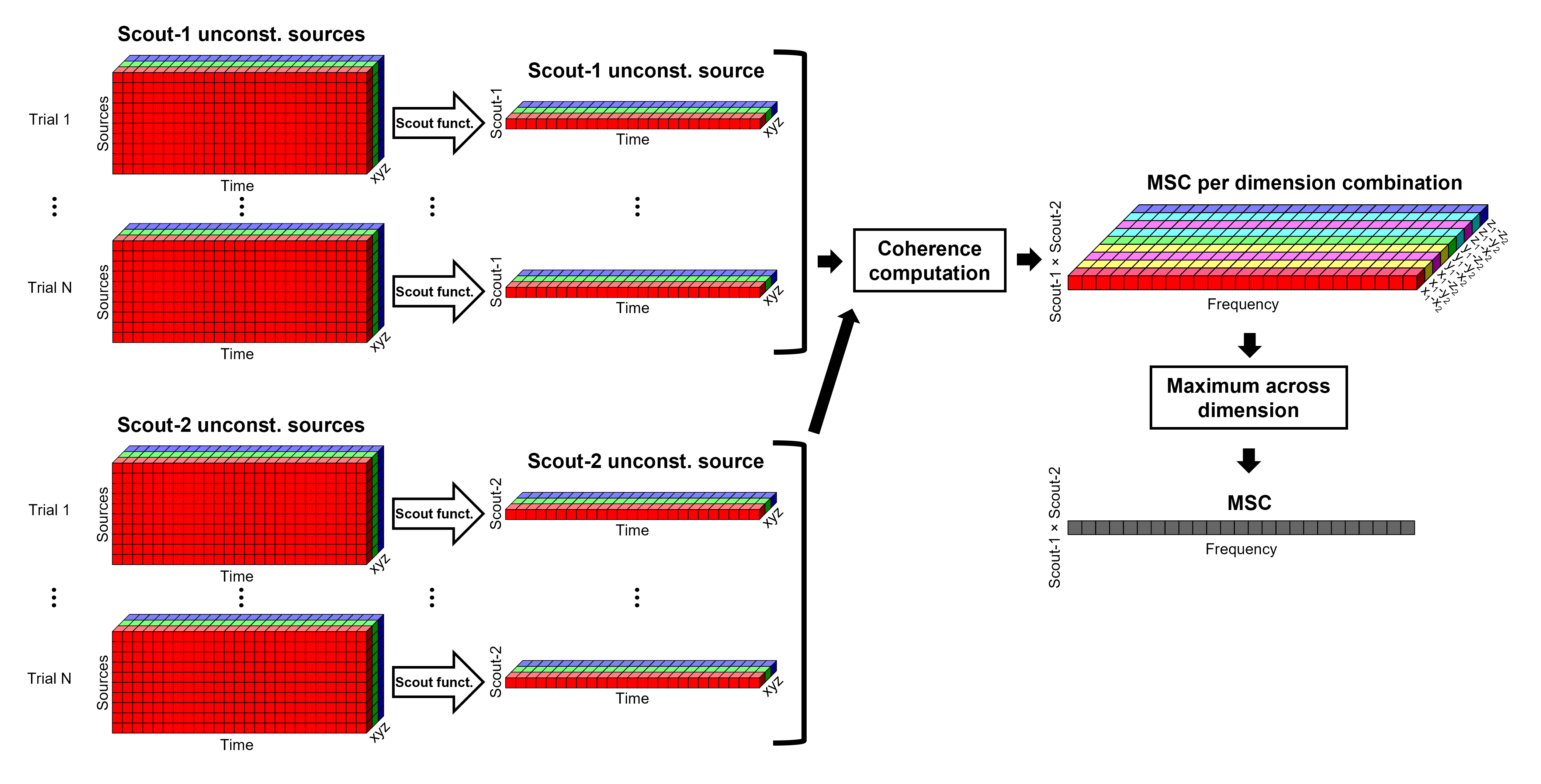
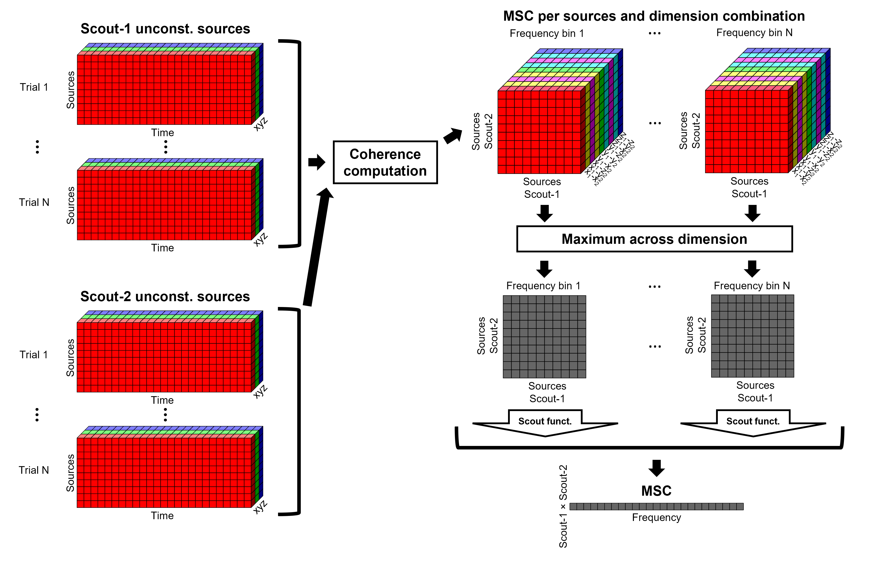
The sections below explain the processing steps for the cases of constrained and unconstrained sources, for coherence between two scouts (Scout-1 and Scout-2). In either case, the outcome is one coherence spectrum per pair of scouts.

Method for constrained sources

The computation steps depend of when the scout function is applied:

• If the scout function is applied before: The scout function (e.g., mean) is applied for all the source time series in each scout; resulting in 1 time series per scout. These scout time series are then used to compute coherence resulting in 1 coherence spectrum per scout.

• If the scout function applied after: coherence is first computed between each combination of souces-scout1 and sources-scout2 resulting in N coherence spectra, with N being the product of sources-scout1 and sources-scout2. Finally the scout function is applied twice (once for each scout) to the resulting coherence spectra to obtain one coherence spectrum per scout pair. This is a considerably more greedy option that the "before" option above, as it computes coherence measures each source in scout1 and each source in scout2. This requires more computing resources; see introduction for an example.

Method for unconstrained sources

As ?described above, when computing coherence with unconstrained sources it is necessary to perform dimension reduction across directions. When this reduction is done by first flattening the unconstrained sources, is performed on unconstrained sources coherence computations is carried out as described in the ?previous section. However, if the sources are not flattened before computing coherence is carried out as follows:

Before: The scout function (e.g., mean) is applied on each direction on the elementary source time series each scout, which results in 3 time series per elementary direction, per scout. These scouts time series are then used to compute coherence measures, yielding to 9 coherence spectra (1x-2x, 1x-2y, 1x-2z, 1y-2x, ..., 1z-2z) for each pair of scouts. The resulting coherence spectra are finally aggregated across the 9 dimensions with maximum per frequency bin, resulting in one single coherence spectrum for each pair of scouts.

After: With this option, coherence is first computed between each pair of source locations (each with 3 time series) in the two scouts, yielding to 9 coherence spectra for each pair of sources in the scouts. Then, these coherence spectra are aggregated across the 9 combinations of dimensions (1x-2x, 1x-2y, 1x-2z, 1y-2x, ..., 1z-2z) to obtain one single coherence spectrum for each pair of sources within the scouts. Finally, the scout function (e.g., mean) is applied twice (once per scout) to the coherence spectra for each source within the scouts to obtain one single coherence spectrum for each pair of scouts. Applying the scout function "after" is a considerably more greedy option that the applying the scout function "before", as it computes coherence measures between all 45000x45000 elementary source signals, and this number is multiplied by the number of frequency bins. This requires more computing resources; see the introduction for an example.

Example

Here, we will compute the coherence from scouts, using mean as scout function with the before option. We will use the Schaefer 100 parcellation atlas on to the orientation-constrained source map.

• Use Search Database () to select the Left trials with their respective (surface)(Constr) source maps, as shown in the previous section.

• In the Process2: Left trial group into both the Files A and Files B boxes. Select Process recordings () for Files A, and Process sources () for Files B.

• 

Open the Pipeline editor:

• Add the process Connectivity > Coherence AxB [2023] with the following parameters:

  • Time window = All file

  • Source channel (A) = EMGlft

  • Check Use scouts (B)

  • From the menu at the right, select Schaefer_100_17net

  • Select all the scouts

  • Scout function: Apply: before

  • Scout function: mean

  • Select Magnitude squared coherence as Connectivity metric

  • Select Fourier transform as Time-freq decomposition method

  • Click in the [Edit] button to set the parameters of the Fourier transform:

    • Select Matlab's FFT defaults as Frequency definition

    • FT window length = 0.5 s

    • FT window overlap = 50%

    • Highest frequency of interest = 80 Hz

  • Time resolution = None

  • Estimate & save = across combined files/epochs

• Add the process File > Add tag with the following parameters:

  • Tag to add = (surface)(Constr)

  • Select Add to file name

• Run the pipeline

Double-click on the new file: the coherence spectra are not displayed on the cortex; they are plotted for each scout. The 1xN connectivity file can also be shown as an image as displayed below:

Note that at 14.65 Hz, the two highest peaks correspond to the SomMotA_4 R and SomMotA_2 R scouts, both located over the right primary motor cortex.

Method for mixed source models

Mixed models refer to source models with multiple regions that may include surface and volume regions, and regions with different source orientation constraints. To compute connectivity between surface and volume regions, you must first create volume scouts for the volume regions of the mixed model, and then use the process2 tab with the same files on both sides. On one side you can select surface scouts, and the other, the volume scouts you created. For connectivity between surface regions only, or volume regions only, use the process1 tab.

Additional documentation

Articles

• Conway BA, Halliday DM, Farmer SF, Shahani U, Maas P, Weir AI, et al.
  Synchronization between motor cortex and spinal motoneuronal pool during the performance of a maintained motor task in man.
  The Journal of Physiology. 1995 Dec 15;489(3):917–24.

• Kilner JM, Baker SN, Salenius S, Hari R, Lemon RN.
  Human Cortical Muscle Coherence Is Directly Related to Specific Motor Parameters.
  J Neurosci. 2000 Dec 1;20(23):8838–45.

• Liu J, Sheng Y, Liu H.
  Corticomuscular Coherence and Its Applications: A Review.
  Front Hum Neurosci. 2019 Mar 20;13:100.

• Sadaghiani S, Brookes MJ, Baillet S.
  Connectomics of human electrophysiology.
  NeuroImage. 2022 Feb;247:118788.

Tutorials

• Tutorial: Functional connectivity

• Tutorial: Source estimation

• Tutorial: Volume source estimation

• Tutorial: Scouts

• Tutorial: Connectivity graphs

Scripting

The following script from the Brainstorm distribution reproduces the analysis presented in this tutorial page: brainstorm3/toolbox/script/tutorial_coherence.m