Brainstorm
  • Comments
  • Menu
    • Attachments
    • Versions
    • Raw Text
    • Print View
  • Login

Software

  • Introduction

  • Gallery

  • Download

  • Installation

Users

  • Tutorials

  • Forum

  • Courses

  • Community

  • Publications

Development

  • What's new

  • What's next

  • About us

  • Contact us

  • Contribute

Revision 3 as of 2025-07-24 18:10:17

SEEG Time-Frequency Fingerprint Analysis for Epileptogenic Zone Localization

Authors: Yash Shashank Vakilna, Chinmay Chinara, Johnson Hampson, Takfarinas Medani, Raymundo Cassani, John Mosher, Sylvain Baillet, Richard Leahy

TODO: Add flowchart

It guides users through computing time-frequency decomposition maps to identify the epileptogenic zone (EZ) using both ictal and interictal SEEG data.

Contents

  1. Access the recordings
    1. Link the recordings
    2. Import the contacts positions
  2. Display the depth electrodes
    1. 3D figures
    2. MRI Viewer
    3. Panel iEEG
  3. Review recordings
    1. Power spectrum
    2. Add events
  4. Import epochs of interest
    1. Import in database
    2. Bipolar montage
  5. Head modeling
  6. Compute noise covariance matrix
  7. Modeling interictal spikes
    1. Compute inverse model
    2. Display sensor time series
    3. View sources
    4. Atlases and scouts
  8. Modeling ictal wave
  9. Modeling ictal onset with LVFA
    1. Sensor space
    2. Source space
  10. Modeling ictal onset with repetitive spiking
    1. Sensor space
    2. Source space
  11. Additional Documentation
    1. Forum discussions
    2. Related tutorials
  12. Scripting

Access the recordings

Link the recordings

  • Switch to the "functional data" view (2nd button, on top of the database explorer).
  • Right-click on the subject folder > Review raw file:

    • Select the file format: EEG: EDF/EDF+

    • Select all the recordings: tutorial_seizure_fingerprinting/recordings/*.edf

      15_import_link.png

    • The selected recordings get added to the database.
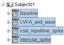
      15_import_link2.png

  • The new files Link to raw file let you access directly the contents of the original SEEG files. The menu Review raw file does not actually copy any data to the database. More details.

Import the contacts positions

In order to generate epileptogenicity maps, we need accurate 3D positions for the contacts of the depth electrodes. Placing the contacts requires a good understanding of the implantation scheme reported by the neurosurgeon, and some skills in reading MRI scans.

  • The channel file "EDF channels" contain the name of the channels, but not their positions. We need to import or edit separately the positions of the SEEG contacts.
  • Click on the [+] next to the four folders, select all the channel files simultaneously.

  • Right-click one channel file > Add EEG positions > From other studies > Implantation
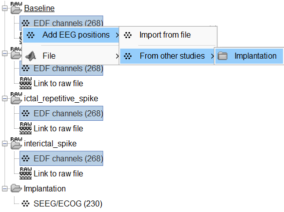
    83_import_pos_file_implantation.png

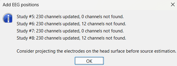
  • At the end, you get a report indicating how many channels from the SEEG recordings were attributed a new 3D position. The channels are matched by name: the position file you import must include the labels of the channels and they must be named exactly in the the same way as in your recordings.
    20_import_pos_report.png

  • For EDF Channels under LVFA_and_wave and interictal_spike, there were 12 channels not found. The type of the channels for which a position was not found is set to EEG_NO_LOC, in order to ignore them when processing the SEEG data. In this example dataset, the channels numbered 245 to 255 and 262 are not found as they are not SEEG contacts.

  • For all the EDF Channels, mark the channel MPS16 as SEEG_NO_LOC because if not marked, when we compute the forward head model using BEM surfaces it says that MPS16 lies outside the BEM layer. Marking it excludes it from any future computations.

  • You should always validate that the type of all the channels has been detected correctly. Check also that the names are correct and using the same convention for all the contact of a given electrode. These are entered manually, and typing errors are frequent. Right-click on a channel file > Edit channel file.

    16_edit_channel.png

  • To edit one channel, double-click on the text to modify. To edit multiple channels, select them all and right-click > Set channel group/type. The column Group corresponds to the name of the depth electrode. It is detected based on the channel type and name. If you include as SEEG a channel that detected as something else or rename a channel, you would need to manually update the channel name.

  • If you don't have the positions for the SEEG contacts, or if they don't look correctly aligned, see the section Edit the contacts positions on how to tackle it.

  • To make this tutorial easier to reproduce and follow, we also distribute the positions of the contacts (that were localized as per the section above) exported as a .tsv file (tutorial_seizure_fingerprinting/recordings/Subject01_electrodes_mm.tsv). To import the contacts position from that refer to Epileptogenicity tutorial.

Display the depth electrodes

3D figures

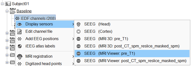
  • Right-click on the channel file > Display sensors and explore all the available options.
    23_display_menu.png

  • You can render the SEEG depth electrodes in 3D together with the subject anatomy: surfaces, pre- or post-implantation volumes. You can add more anatomy elements to the figure with the button Add a surface ( [ATTACH] ) at the top-right of the Surface tab. For more help: Display the anatomy.
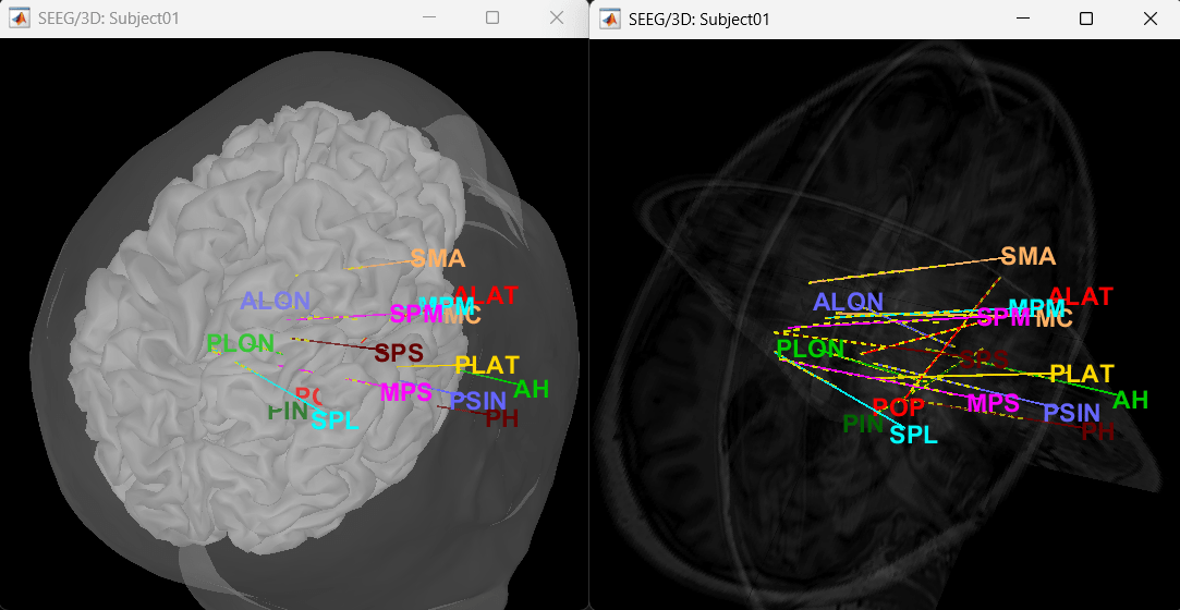
    24_display_3d.png

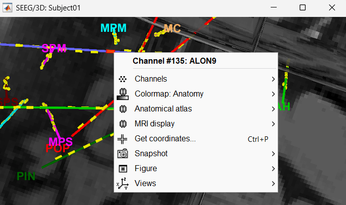
  • Click on a contact to select it, right-click on it to get its name.
    25_display_selectchan.png

MRI Viewer

  • You can also display the contacts in the MRI viewer, on top of the the pre- or post-implantation volumes. By default, the electrode is displayed in a slice if there is a SEEG contact associated to it in the slice.
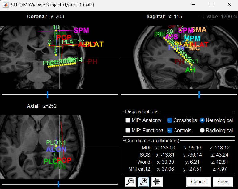
    26_display_mri.png

  • To display all the electrodes, select the option "MIP: Functional". For a glass-brain view, select at the same time the option "MIP: Anatomy".
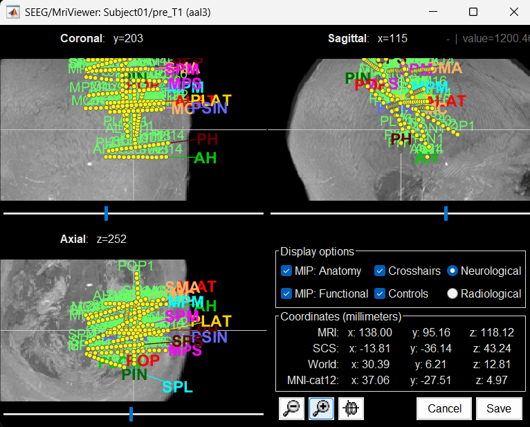
    27_display_mri_mip.png

  • Zoom in/out with the buttons or the associated shortcuts (Ctrl+Scroll or +/-) and explore the volume with (Shift+)x/y/z. Additional display options are available in the popup menu for this figure. All the shortcuts are listed in this tutorial.

Panel iEEG

  • When opening SEEG/ECOG recordings, the panel iEEG is added to the Brainstorm window. You can use it to edit the display properties of the depth electrodes. More details about the iEEG Panel can be found in the Epileptogenicity tutorial.
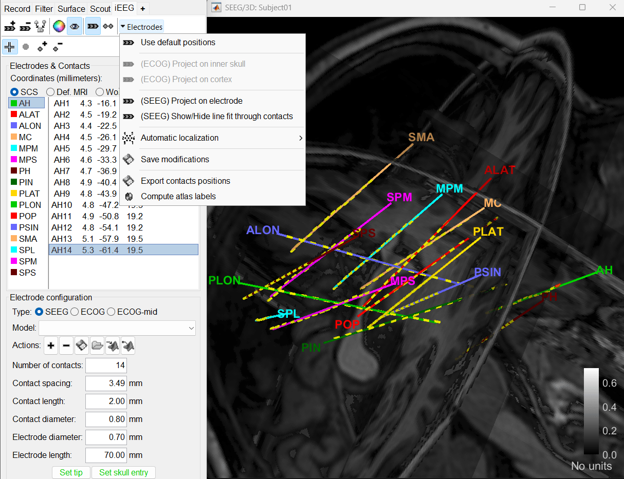
    29_panel_ieeg.png

To know more about ways to display the SEEG recordings in Brainstorm refer to the Epileptogenicity tutorial.

Review recordings

Power spectrum

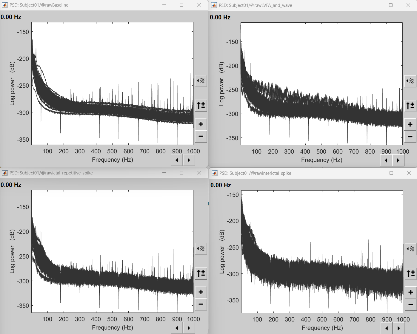
We recommend that you start your data analysis with a power spectral density estimation of the recordings to check the quality of sensor recording. This is described in more details in the Power spectrum tutorial.

  • In Process1, select all the continuous files (Link to raw files or folders).
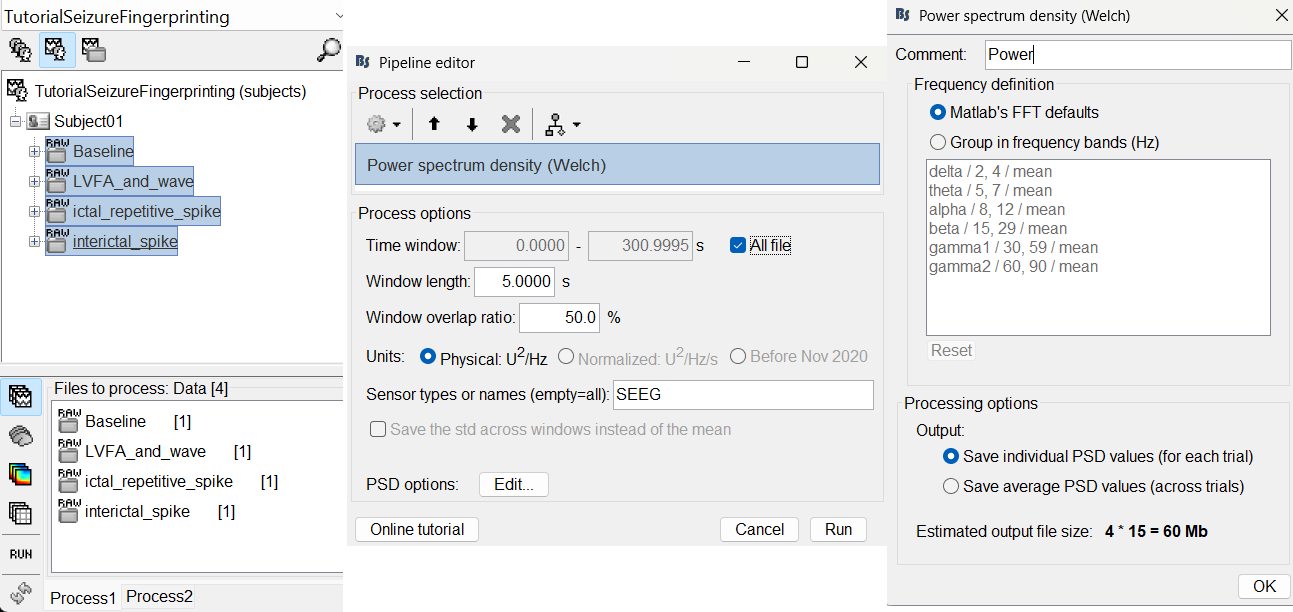
    48_psd_process.png

  • Double-click on the PSD files to display them. It can be seen that the power line interference at 60Hz along with its harmonics have been removed. This was done using a notch filter. More details can be found in the notch filter section in the above tutorial.
    49_psd_result2.png

Add events

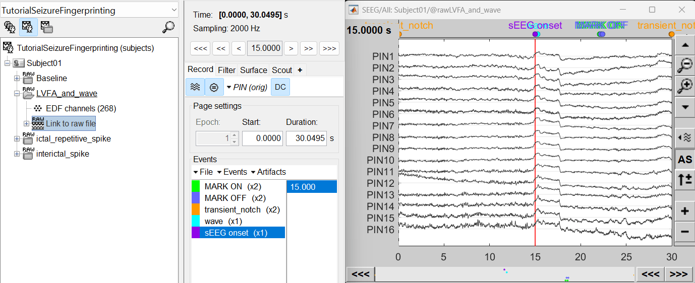
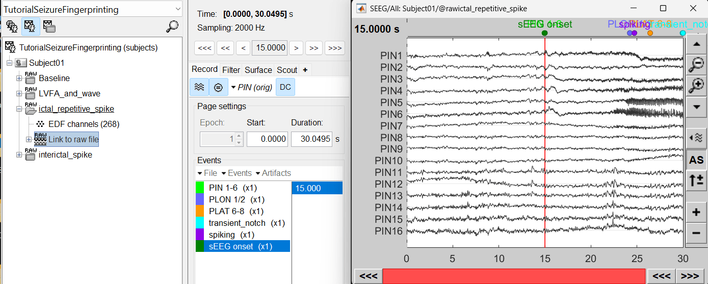
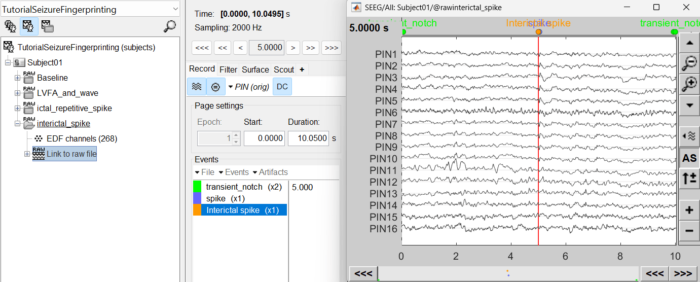
We need to mark seizure onset event for the ictal and LVFA and wave recordings and spike event for interictal recording. There are events already available in recordings, that were marked for clinical use, to jump quickly to the page of interest. More details can be found in the tutorial Event Markers.

  • For LVFA and wave, we will create a new event sEEG Onset at around 15s (center of the 30s recording extract).
    51_mark_onset_law.png

  • For ictal repetitive spike, we will create a new event sEEG Onset at around 15s (center of the 30s recording extract).
    50_mark_onset_irs.png

  • For interictal spike, we will create a new event Interictal spike at around 5s (center of the 10s recording extract).
    52_mark_spike_is.png

Import epochs of interest

At this point of the analysis, we are still looking at the original files, no SEEG data was copied to the database. The montages are saved in the Brainstorm preferences, the new events are saved in the links of the database.

We are now going to import the three segment of recordings i.e. LVFA and wave , ictal repetitive spike and interictal spike which are a subset of the Baseline recording.

Import in database

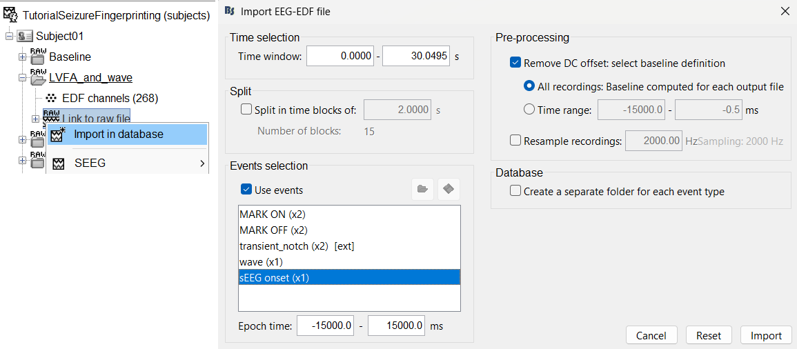
  • Right click on LVFA_and_wave > Link to raw file > Import in database.

    • Time window: All (0 to 30.0495)
    • Split in time blocks: Disabled
    • Use events: Enabled, select sEEG Onset

    • Epoch time: [-15000, +15000] ms (imports -15s to 15s around the event sEEG Onset)

    • Remove DC offset: Enabled. More details can be found here.

    • Resample: Disabled
    • Create a separate folder for each event type: Disabled
    • Click Import.

      53_import_onset.png

  • Repeat the same steps above for importing ictal repetitive spike into the database.

  • Repeat the same steps above for importing interictal spike into the database with the modification in the following options:

    • Time window: All (0 to 10.0495)
    • Use events: Enabled, select Interictal spike

    • Epoch time: [-5000, +5000] ms (imports -5s to 5s around the event Interictal spike)

  • At the end, you should have three new folders LVFA and wave , ictal repetitive spike and interictal spike, the same name as the original raw files, but without the tag RAW on top. These new folders contain copies of the SEEG recordings, if you delete these folders from the database explorer, you lose the recordings they contain.

  • The imported epochs are saved with a new timing: for LVFA and wave and ictal repetitive spike, the reference time t=0s is now the event sEEG Onset and for Interictal spike, the reference time t=0s is now the event Interictal spike, which has been removed from the list. You can still see the other marker timings adjusted accordingly.
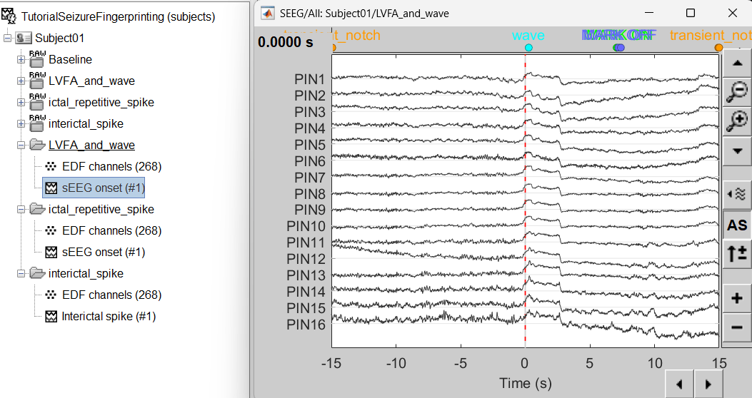
    54_import_database.png

Bipolar montage

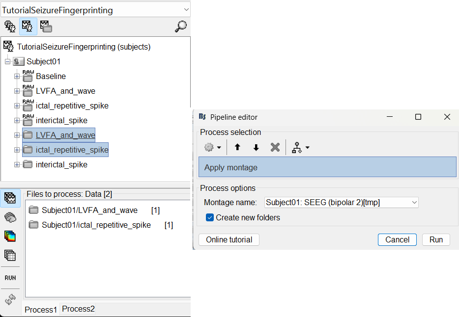
We will run the rest of the analysis using a bipolar montage (bipolar-2). The montage selected in the Record tab is for visualization only, most processes ignore this selection and work only on the original common-referential montage. To compute bipolar montage on time series, we need to explicitly apply the montage to the recordings. More details can be found in tutorials Montage editor and Epileptogenicity.

  • In Process1, drag and drop all the imported recordings (either the folders or the files).

  • Run the process Standardize > Apply montage

    • Montage name: Subject01: SEEG (bipolar 2)[tmp]

    • Create new folders: Enabled

      55_import_montage.png

  • This process rewrites the channel files and data files in the selected folders. The position associated with a bipolar channel in the channel file is the middle of the segment between the two contacts (e.g. AH1-AH2 is placed half-way between AH1 and AH2).
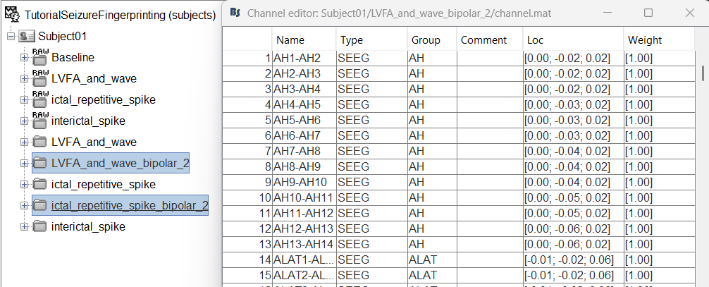
    56_import_montage_chan.png

Head modeling

The forward models depend on the subject's anatomy, including head size and geometry, tissue conductivity, the computational method, and sensor characteristics. In this section, we will use the Boundary Element Method (BEM) approach available in Brainstorm for constructing the head model for sEEG.

  • We will first generate the BEM head surfaces from the MRI. More details can be found in OpenMEEG BEM tutorial. This will generate three surfaces head, outer skull and inner skull estimated from the head mask and the cortex obtained from the segmentation. The BEM surfaces will be used for the BEM forward computation below.
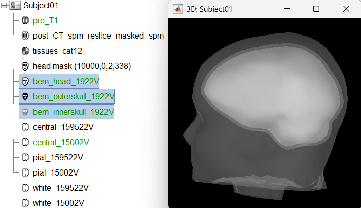
    57_head_modeling.png

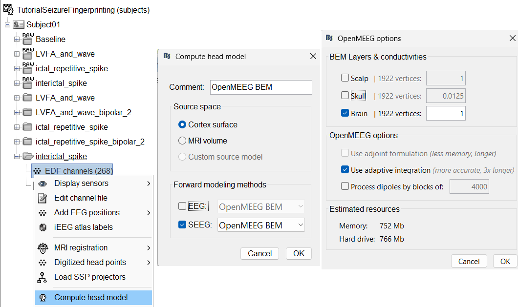
  • We will then compute the forward head model using the OpenMEEG BEM method. Switch to functional tab, right-click on the interictal_spike > EDF channels > Compute head model.

    • Source space: Cortex surface

    • Forward modelling methods: SEEG: OpenMEEG BEM

    • Use only Brain in BEM layers and conductivities (corresponds to bem_innerskull surface) as other surfaces do not matter for SEEG.

    • Use default OpenMEEG options.

      58_headmodeller_openmeeg.png

  • A new head model will be added to the folder.
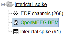
    59_headmodeller_final.png

  • Right click on the head model file > Copy to other folders. Since the other folders contain data collected from the same subject using the same set of electrodes, we do not need to recompute the head model for each of them separately.

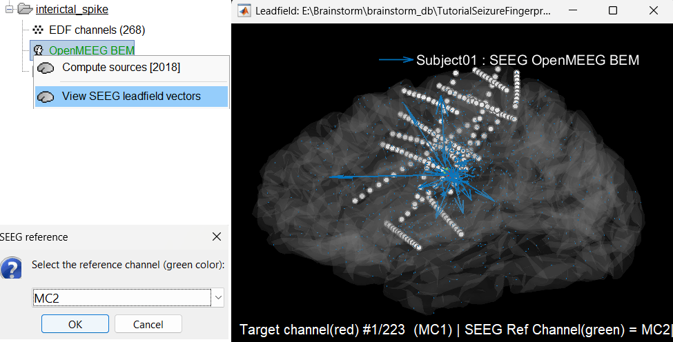
  • View leadfield vectors:

    • Right click on the head model file > View SEEG leadfield vectors

    • Select reference MC2 and click OK

    • Click on the figure and press E to display the electrodes

    • Make sure scouts are unselected (Scout tab > ALL and SEL unselected)

    • Surface tab: transparency = 90 and press Shift+Up arrow till the arrows are visible. Press Up/down to change the Reference electrode, Right/Left to change the target. Close all figures once done.
      60_leadfield_vector.png

Compute noise covariance matrix

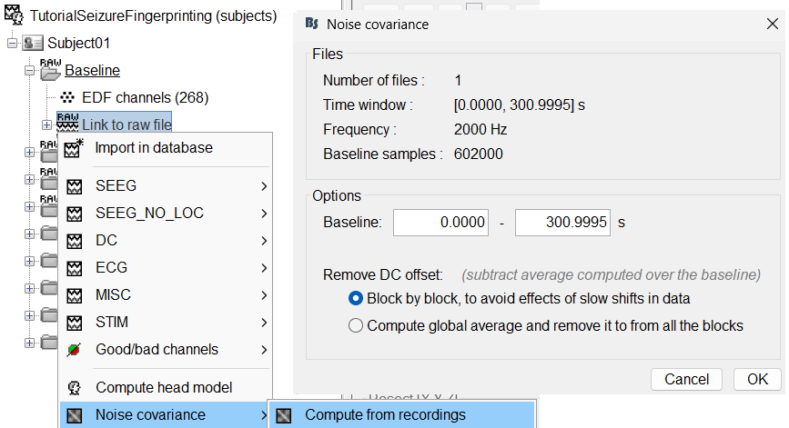
  • We will compute the noise covariance matrix for the Baseline recording as per the tutorial Noise covariance.

  • Right click on the Baseline (RAW) > Link to raw file > Noise covariance > Compute from recordings . Keep the default values and click OK.
    61_noise_covariance.png

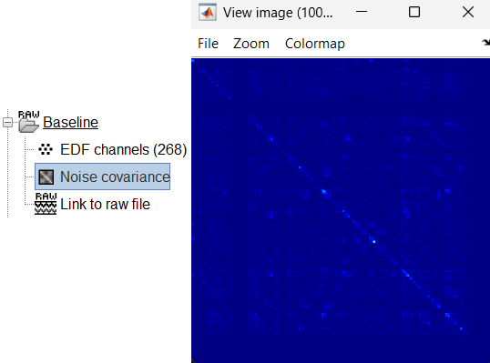
  • Noise covariance node gets added to the database.
    61_noise_covariance2.png

  • Right click on the Noise covariance and Copy to other folders.

Modeling interictal spikes

Compute inverse model

  • We will compute the inverse model for the interictal_spike recording. For more details refer to the tutorials Source estimation and Volume source estimation.

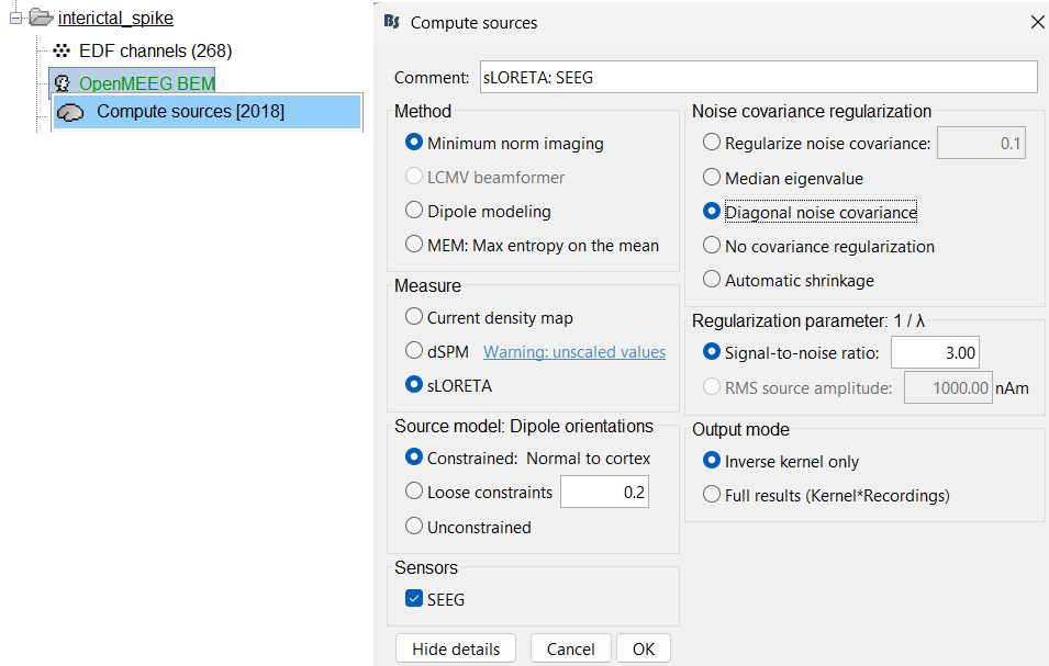
  • Expand the interictal_spike folder, right click on OpenMEEG BEM > Compute sources [2018].

    • Method: Minimum norm imaging

    • Measure: sLORETA

    • Source model: Dipole orientations: Constrained: Normal to cortex

    • Noise covariance regularization: Diagonal noise covariance

    • Regularization parameter: Signal-to-noise ratio: 3.00

    • Output mode: Inverse kernel only
    • Sensors: SEEG. Click OK.

      62_inverse_model1.png

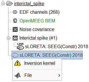
  • Two files get added to database. To learn about inversion kernel and LINK files in database refer to this section.
    62_inverse_model2.png

Display sensor time series

  • Display time series

    • Right-click on recording Interictal spike > SEEG > Display time series

    • On the Record tab, select montage SPS (bipolar 2)

    • Select the first peak of SPS10-SPS11 (Time 0.041s).

  • Display 2D layout of the spike

    • Right-click on recording Interictal spike > SEEG > 2D Layout

    • Click [...] on the corner and set[-500, 500] as the time window. Doing this will enable visualizing 1s of data across all the sensors giving a more clear sense of where the different spikes are.
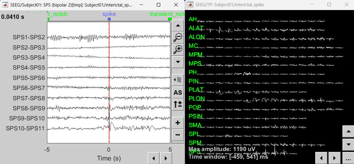
      63_disp_ts_interictal.png

View sources

  • Display on cortex

    • Right click on sLORETA (LINK) > Cortical activations > Display on cortex

    • Show sensors: Ctrl+L (electrodes)

    • Set colormap: Colorbar > Colormap:Sources > Permanent menu, select Maximum: Global, Contrast -0, Brightness 0

    • Switch to Surface tab: Amplitude 26%, Min size 13
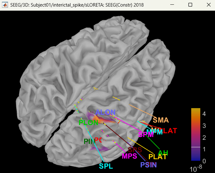
      64_view_inv_model_cortex.png

  • Display on 3D MRI viewer

    • Right click on sLORETA (LINK) > Cortical activations > Display on MRI (3D)

    • Show sensors: Ctrl+L (electrodes)

    • Press M to go to voxel with maximum intensity
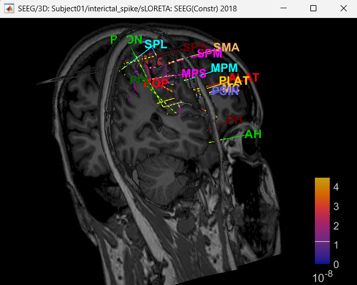
      65_view_inv_model_mri3d.png

  • Display on MRI viewer

    • Right click on sLORETA (LINK) > Cortical activations > Display on MRI (MRI Viewer)

    • Turn on MIP: Functional

    • Switch to Surface tab, Amplitude: 56%, and press M to select voxel with maximum intensity
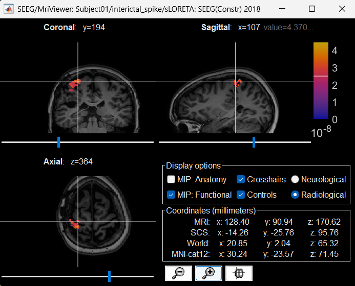
      66_view_inv_model_mri.png

Atlases and scouts

  • Display sources on the cortical surface
    • Right click on sLORETA (LINK) > Cortical activations > Display on Cortex

    • In the Scout tab, use the drop box to select Desikan-Killiany and click on ALL. This atlas is provided by default in Brainstorm. Ctrl+L to show all electrodes.
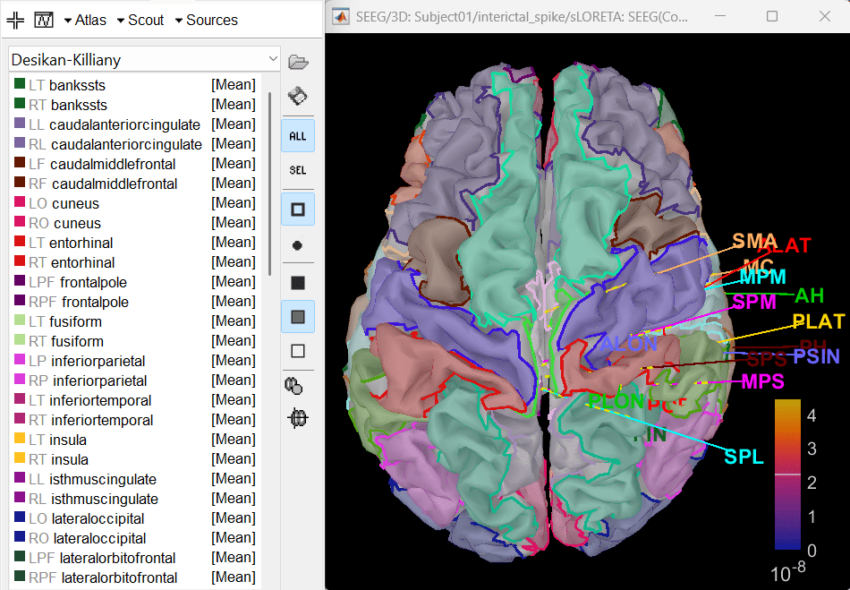
      67_atlas_dk.png

  • Since all the electrodes in the data are implanted on the right hemisphere of the brain, it is better to edit this atlas to only have scouts defined for the right region and remove the rest. Also we can subdivide the atlas to smaller scout regions to have smaller ROIs that will help in having better and more focused time-frequency epileptogenic maps later in the tutorial.
    • In Scout tab, select all the scouts in the right hemisphere and then create a new atlas from the selected scouts by Atlas > New atlas > Copy selected scouts. It will create a new atlas named Desikan-Killiany_02. Rename it to Desikan-Killiany_RH where "RH" indicates right hemisphere.

    • Atlas > Subdivide atlas > Area > Area of the sub-regions: 5 (cm sq.). A total of 176 scouts will be created with smaller and more focused ROI.
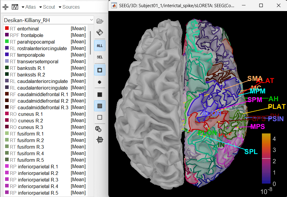
      68_atlas_dk_176.png

  • To know more about scouts in Brainstorm refer to the tutorial Scouts.

Modeling ictal wave

Switch to the folder LVFA_and_wave (not the RAW folder) and repeat the steps to compute inverse model as per the section above and study the sensor time series and inverse modeling results.
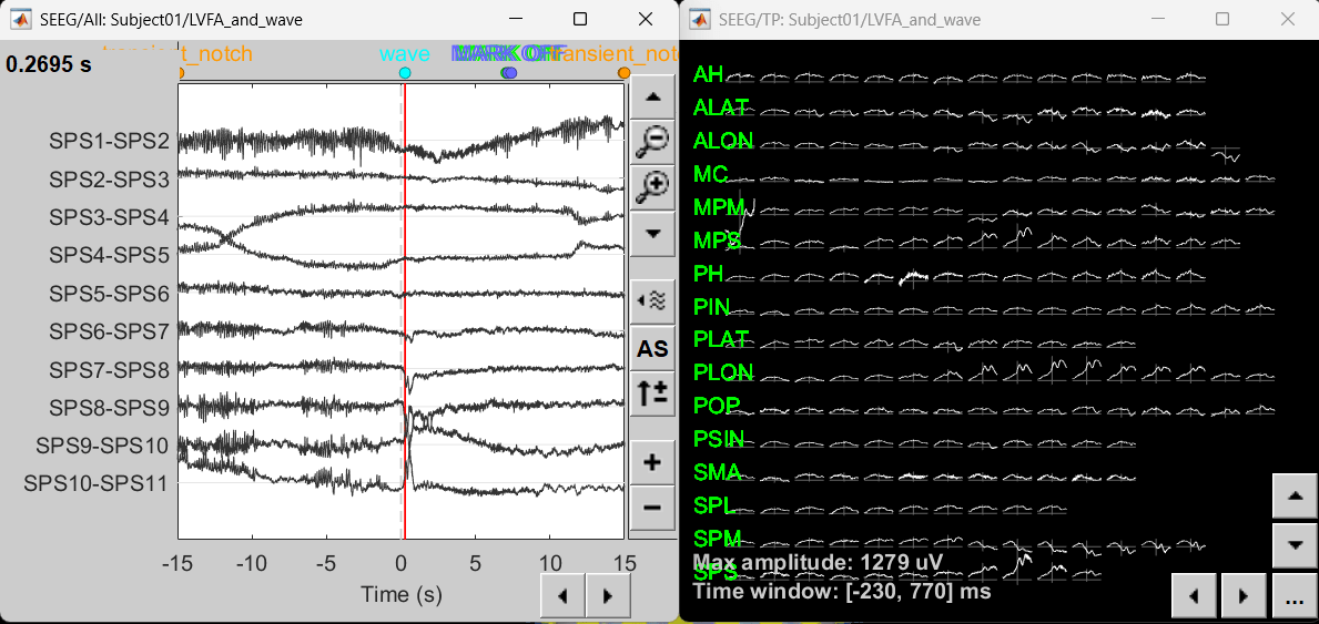
69_disp_ts_wave.png

70_view_inv_model_wave.png

Modeling ictal onset with LVFA

Sensor space

Compute time-frequency decomposition

  • Navigate and expand LVFA_and_wave_bipolar_2 folder

  • Delete any previous recordings in the Process 1 tab below

  • Drag-and-drop recording file sEEG onset (#1) | bipolar 2 in Process 1, click [RUN]
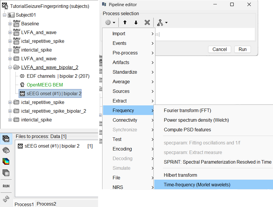
    71_time_freq_decomp_lvfa1.png

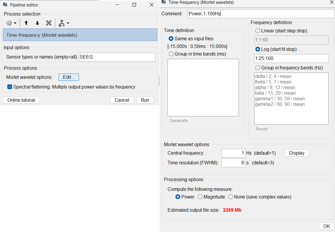
  • Add the process: Frequency > Time-frequency (Morlet wavelets)

    • Sensor type: SEEG

    • Select Spectral flattening: Multiply output power values by frequency

    • Click Edit...

    • Frequency definition: Log (start:N:stop), 1:25:100

    • Central Frequency: 1 Hz, Time resolution (FWHM): 6s. Click OK and Run.
      71_time_freq_decomp_lvfa2.png

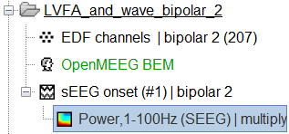
  • A new node Power,1-100Hz (SEEG) | multiply gets added to the database.
    71_time_freq_decomp_lvfa3.png

  • For more details go through the tutorial Time-frequency.

View time-frequency maps

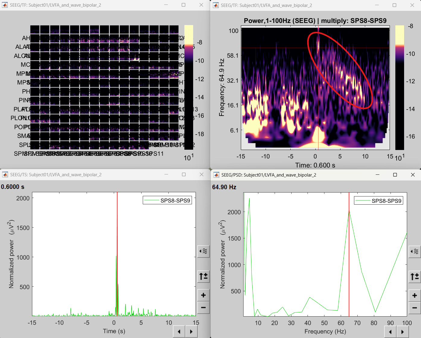
  • Right click sEEG onset (#1) | bipolar 2 > Power,1-100Hz (SEEG) | multiply > All channels

  • Click on Log(Power) to bring out the essential features in the maps.

  • Click on Smooth display to apply a Gaussian kernel to the map so that the underlying pattern becomes clearer for viewing.

  • Click on SPS8-SPS9

  • Set colormap: right-click on Colorbar > Colormap: Timefreq > Permanent menu, Turn-off [Absolute Value](if on), Maximum: Local, Contrast 49 Brightness -65

  • Right-click on the colored time-frequency plot > Power Spectrum, Time Series
    72_time_freq_map_lvfa.png

  • The red marked area above is the high frequency activity. The bottom right area contains the pre-ictal spikes that is signature of seizure fingerprinting.

Source space

Extract scout time series

  • We are going to now extract a single time-series for each of these scouts that best defines it.
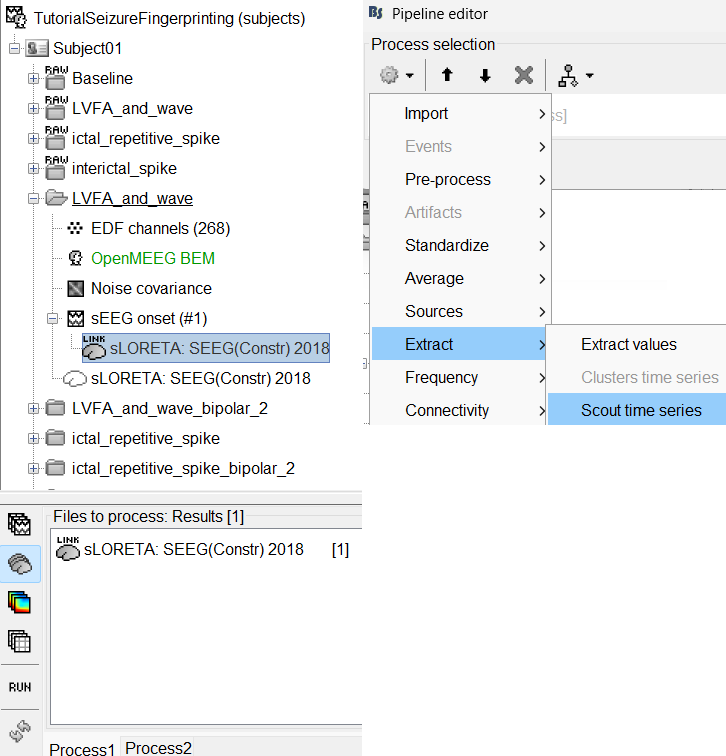
  • Switch to the folder LVFA_and_wave (not the RAW folder).

  • Drag-and-drop sLORETA: SEEG(Constr) 2018 (LINK) in Process 1, click [RUN]
    73_scout_time_series_lvfa1.png

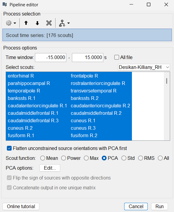
  • Add the process: Extract > Scout time series

    • Select Desikan-Killiany_RH.

    • Select scouts: Press Ctrl+A to select all the scouts in the box.

    • Select Scout function: PCA

    73_scout_time_series_lvfa2.png

  • A new matrix file sEEG onset (#1) | 176 scouts gets added to the database.
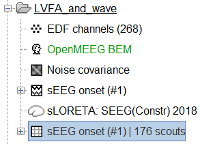
    73_scout_time_series_lvfa3.png

  • Right click on matrix file sEEG onset (#1) | 176 scouts > Display as time series.
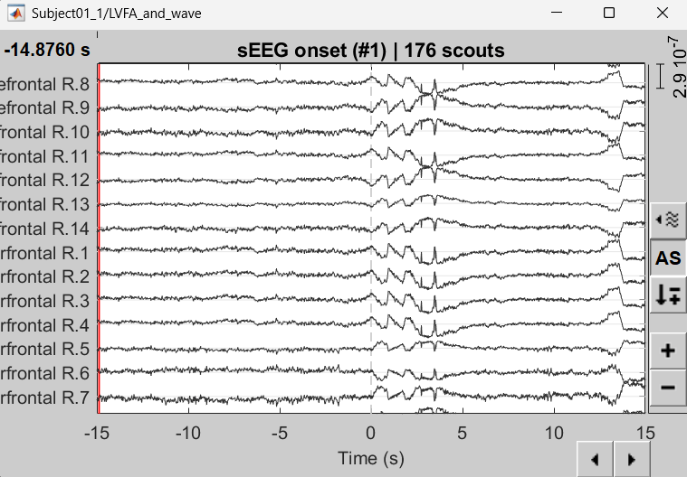
    75_scout_time_series_lvfa2.png

Compute time-frequency decomposition

  • Drag-and-drop matrix file sEEG onset (#1) | 176 scouts in Process 1, click [RUN]

  • Rest of the steps are the same as the corresponding earlier section in sensor space.
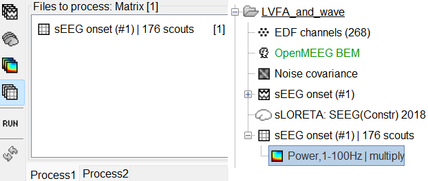
    74_time_freq_decomp_lvfa2.png

View time-frequency maps

  • Right click on matrix file sEEG onset (#1) | 176 scouts > Power,1-100Hz | multiply > Time-freq: All matrices

  • Right click on matrix file sEEG onset (#1) | 176 scouts > Power,1-100Hz | multiply > Time-freq: One matrix. Set selected data as postcentral R.3.

  • Click on Log(Power), Smooth display.

  • Set colormap: right-click on Colorbar > Colormap: Timefreq > Permanent menu, Turn-off [Absolute Value](if on), Maximum: Local, Contrast 52 Brightness -63

  • Right-click on the colored time-frequency plot > Power Spectrum, Time Series
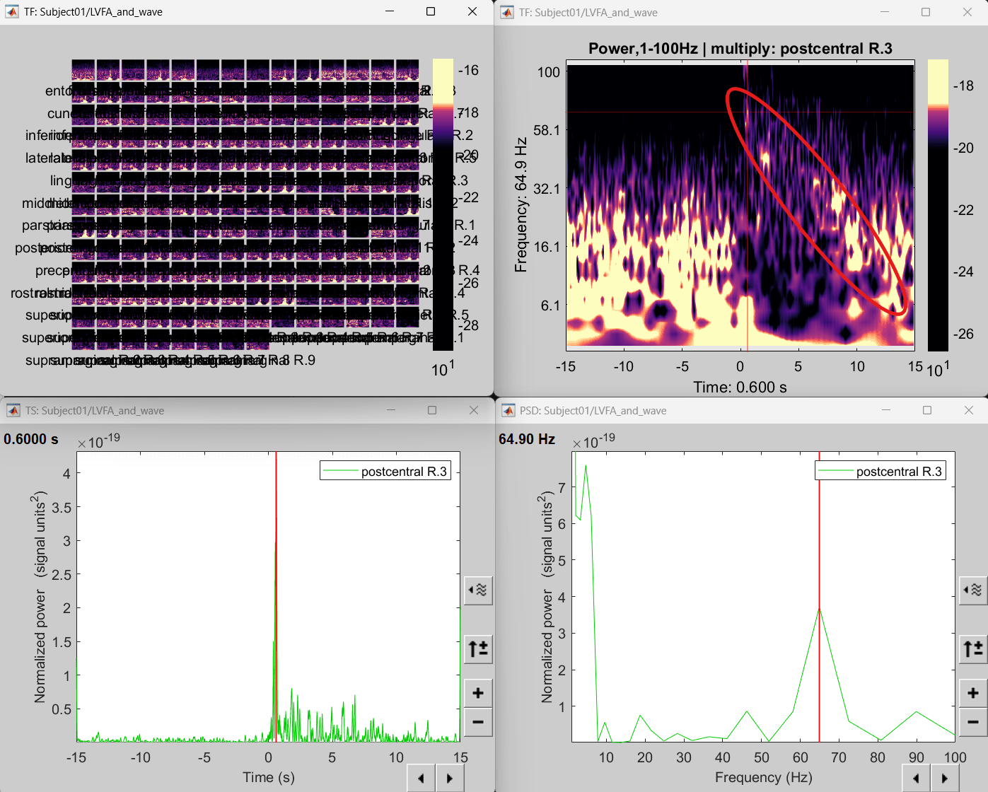
    76_time_freq_map_lvfa2.png

  • The red marked area above is the high frequency activity. The bottom right area contains the pre-ictal spikes that is signature of seizure fingerprinting. We can say that this patch of cortex postcentral R.3 was most associated with the LVFA pattern.

Modeling ictal onset with repetitive spiking

Sensor space

Display time-series

  • Expand the folder ictal_repetitive_spike_bipolar_2

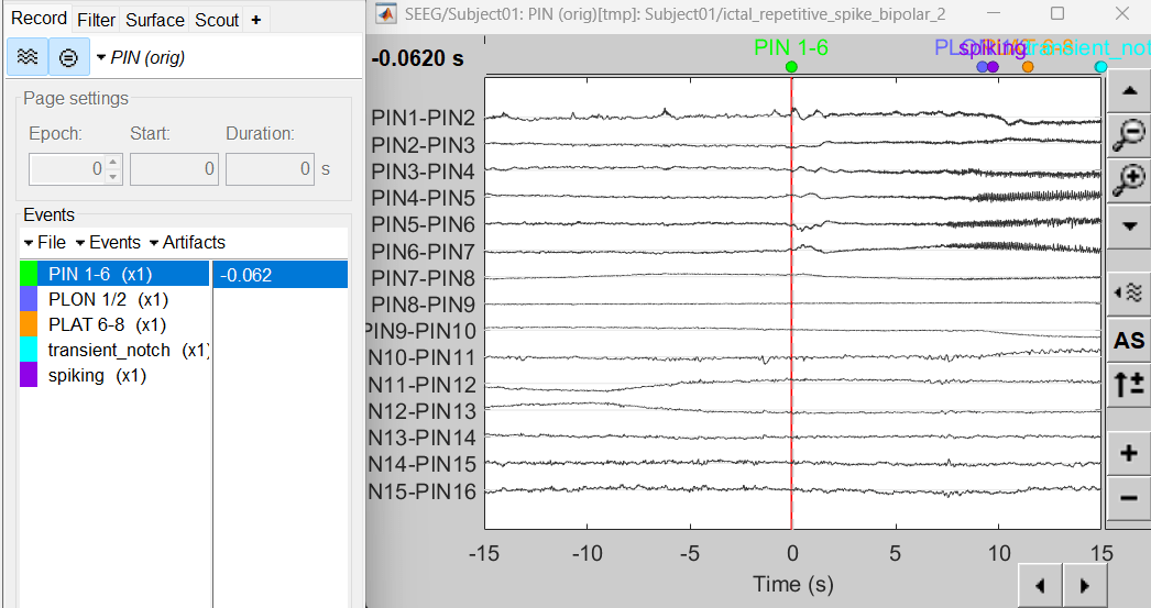
  • Right click on sEEG onset (#1) | bipolar 2 > Display time series

  • Change Montage to PIN > PIN (orig)

    77_time_series_ictal.png

Compute time-frequency decomposition

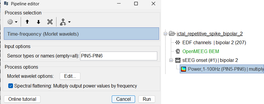
Same as above sections. Only one change, set sensor type: PIN5-PIN6 for Time-frequency (Morlet wavelets) process.
78_time_freq_decomp_ictal.png

View time-frequency maps

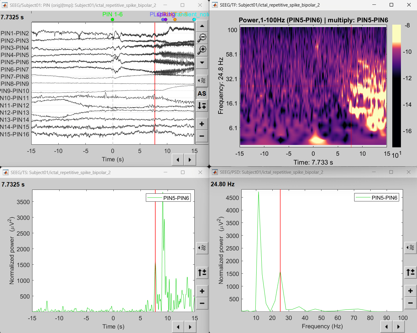
  • Right click on file sEEG onset (#1) | bipolar 2 > Power,1-100Hz (PIN5-PIN6) | multiply > One channel.

  • Click on Log(Power), Smooth display.

  • Set colormap: right-click on Colorbar > Colormap: Timefreq > Permanent menu, Maximum: local, Contrast 23 Brightness -60
    79_time_freq_map_ictal.png

  • The high frequency activity on the right is due to the rhythmic activity seen in the time series for PIN5-PIN6. On analyzing the time-frequency map, this activity is localized between 5Hz and 55Hz. So we need to filter this frequency range so that our results are more focused on the rhythmic activity.

Source space

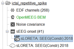
Compute inverse model

  • Switch to the folder ictal_repetitive_spike

  • Repeat the steps as in the previous section.
    80_inverse_model_ictal.png

View sources

  • Right-click on sEEG onset (#1) > SEEG > Display time series.

  • Change Montage to PIN(orig)

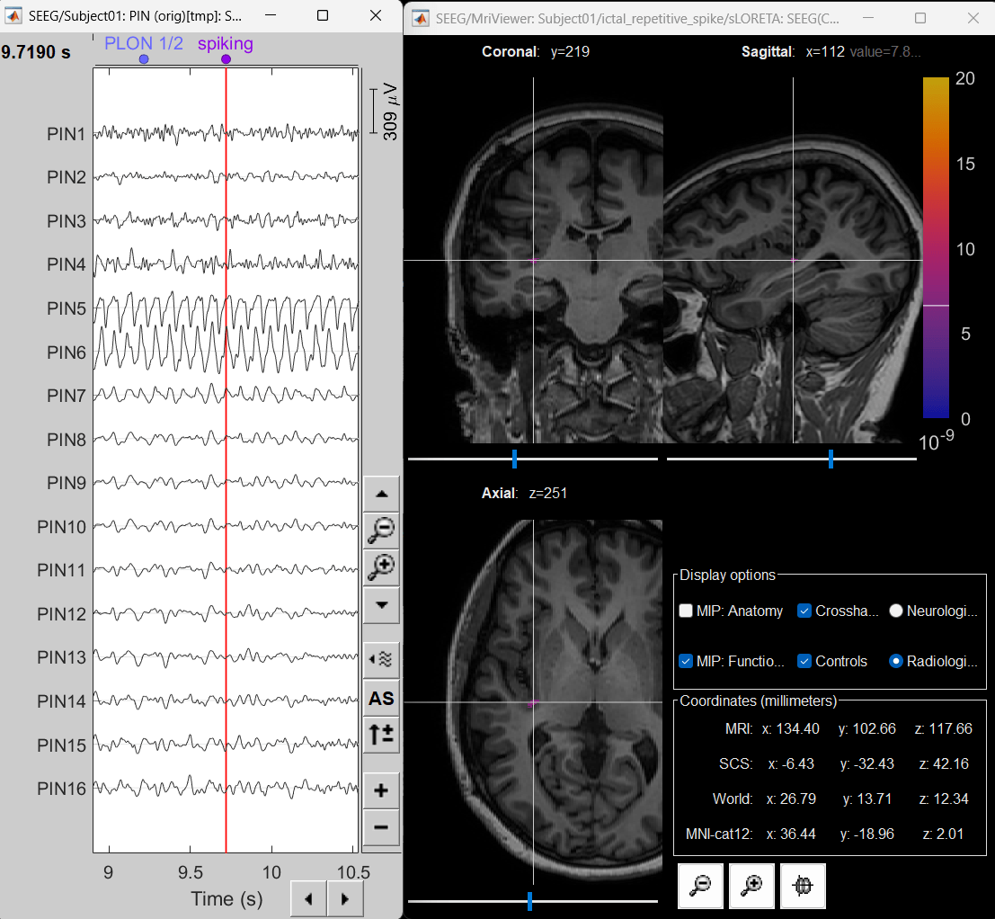
  • Set frequency filter: High-pass: 5Hz, Low-pass: 55Hz

  • Display sources on MRI viewer

    • Right-click on sLORETA: SEEG(Constr) 2018 (LINK) > Cortical activations > Display on MRI (MRI Viewer)

    • Set colormap: Right Click on Colorbar > Colormap: Sources > Permanent Menu, Maximum: Custom [0, 2]

    • Click on Surface tab, set Amplitude 33%
      81_inverse_model_res_ictal.png

  • The peak of the rhythmic activity localized on the patch of the cortex as seen in the MRI Viewer above.

Additional Documentation

Forum discussions

  • Updating SEEG coordinates

Articles

  • Yash Shashank Vakilna, Deniz Atilgan, Johnson Hampson, Chinmay Chinara, Takfarinas Medani, Richard M. Leahy, Nuria Lacuey, Samden D. Lhatoo, Sandipan Pati, John C. Mosher, Jay R. Gavvala.
    Time-Frequency Fingerprint Analysis in SEEG Source-Space to Identify the Epileptogenic Zone.
    Annals of Clinical and Translational Neurology 2025.

Related tutorials

  • Epileptogenicity

  • ECoG/sEEG tutorial

Advanced

Scripting

The following script from the Brainstorm distribution reproduces the analysis presented in this tutorial page: brainstorm3/toolbox/script/tutorial_seizure_fingerprinting.m

1 function tutorial_seizure_fingerprinting(tutorial_dir, reports_dir) 2 % TUTORIAL_SEIZURE_FINGERPRINTING: Script that reproduces the results of the online tutorial "Seizure Fingerprinting". 3 % 4 % CORRESPONDING ONLINE TUTORIALS: 5 % https://neuroimage.usc.edu/brainstorm/Tutorials/SeizureFingerprinting 6 % 7 % INPUTS: 8 % - tutorial_dir : Directory where the tutorial_seizure_fingerprinting.zip file has been unzipped 9 % - reports_dir : Directory where to save the execution report (instead of displaying it) 10 11 % @============================================================================= 12 % This function is part of the Brainstorm software: 13 % https://neuroimage.usc.edu/brainstorm 14 % 15 % Copyright (c) University of Southern California & McGill University 16 % This software is distributed under the terms of the GNU General Public License 17 % as published by the Free Software Foundation. Further details on the GPLv3 18 % license can be found at http://www.gnu.org/copyleft/gpl.html. 19 % 20 % FOR RESEARCH PURPOSES ONLY. THE SOFTWARE IS PROVIDED "AS IS," AND THE 21 % UNIVERSITY OF SOUTHERN CALIFORNIA AND ITS COLLABORATORS DO NOT MAKE ANY 22 % WARRANTY, EXPRESS OR IMPLIED, INCLUDING BUT NOT LIMITED TO WARRANTIES OF 23 % MERCHANTABILITY AND FITNESS FOR A PARTICULAR PURPOSE, NOR DO THEY ASSUME ANY 24 % LIABILITY OR RESPONSIBILITY FOR THE USE OF THIS SOFTWARE. 25 % 26 % For more information type "brainstorm license" at command prompt. 27 % =============================================================================@ 28 % 29 % Authors: Chinmay Chinara, 2025 30 % Yash Shashank Vakilna, 2025 31 % Raymundo Cassani, 2025 32 33 %% ===== PARSE INPUTS ===== 34 % Output folder for reports 35 if (nargin < 2) || isempty(reports_dir) || ~isfolder(reports_dir) 36 reports_dir = []; 37 end 38 % You have to specify the folder in which the tutorial dataset is unzipped 39 if (nargin == 0) || isempty(tutorial_dir) || ~file_exist(tutorial_dir) 40 error('The first argument must be the full path to the tutorial dataset folder.'); 41 end 42 43 %% ===== FILES TO IMPORT ===== 44 % Build the path of the files to import 45 tutorial_dir = bst_fullfile(tutorial_dir, 'tutorial_seizure_fingerprinting'); 46 MriFilePre = bst_fullfile(tutorial_dir, 'anatomy', 'pre_T1.nii.gz'); 47 CtFilePost = bst_fullfile(tutorial_dir, 'anatomy', 'post_CT.nii.gz'); 48 BaselineFile = bst_fullfile(tutorial_dir, 'recordings', 'Baseline.edf'); 49 IctalFile = bst_fullfile(tutorial_dir, 'recordings', 'ictal_repetitive_spike.edf'); 50 InterictalFile = bst_fullfile(tutorial_dir, 'recordings', 'interictal_spike.edf'); 51 LvfaFile = bst_fullfile(tutorial_dir, 'recordings', 'LVFA_and_wave.edf'); 52 ElecPosFile = bst_fullfile(tutorial_dir, 'recordings', 'Subject01_electrodes_mm.tsv'); 53 % Check if the folder contains the required files 54 if ~file_exist(BaselineFile) 55 error(['The folder ' tutorial_dir ' does not contain the folder from the file tutorial_seizure_fingerprinting.zip.']); 56 end 57 % Subject name 58 SubjectName = 'Subject01'; 59 60 %% ===== CREATE PROTOCOL ===== 61 % The protocol name has to be a valid folder name (no spaces, no weird characters...) 62 ProtocolName = 'TutorialSeizureFingerprinting'; 63 % Start brainstorm without the GUI 64 if ~brainstorm('status') 65 brainstorm nogui 66 end 67 % Delete existing protocol 68 gui_brainstorm('DeleteProtocol', ProtocolName); 69 % Create new protocol 70 gui_brainstorm('CreateProtocol', ProtocolName, 0, 0); 71 % Start a new report 72 bst_report('Start'); 73 % Reset visualization filters 74 panel_filter('SetFilters', 0, [], 0, [], 0, [], 0, 0); 75 % Reset colormaps 76 bst_colormaps('RestoreDefaults', 'timefreq'); 77 bst_colormaps('RestoreDefaults', 'source'); 78 % Set the current time series display mode to 'column' 79 bst_set('TSDisplayMode', 'column'); 80 % Hide scouts 81 panel_scout('SetScoutShowSelection', 'none'); 82 83 %% ===== IMPORT MRI AND CT VOLUMES ===== 84 % Create subject 85 [~, iSubject] = db_add_subject(SubjectName, [], 0, 0); 86 % Import MRI volume 87 DbMriFilePre = import_mri(iSubject, MriFilePre, 'ALL', 0, 0, 'pre_T1'); 88 % Set fiducials in MRI coordinates 89 NAS = [104, 207, 85]; 90 LPA = [ 26, 113, 78]; 91 RPA = [176, 113, 78]; 92 figure_mri('SetSubjectFiducials', iSubject, NAS, LPA, RPA, [], [], []); 93 94 % Process: Segment MRI with CAT12 95 bst_process('CallProcess', 'process_segment_cat12', [], [], ... 96 'subjectname', SubjectName, ... 97 'nvertices', 15000, ... 98 'tpmnii', {'', 'Nifti1'}, ... 99 'sphreg', 1, ... % Use spherical registration 100 'vol', 0, ... % No volume parcellations 101 'extramaps', 0, ... % No additional cortical maps 102 'cerebellum', 0); 103 104 % Import CT volume 105 DbCtFilePost = import_mri(iSubject, CtFilePost, 'ALL', 0, 0, 'post_CT'); 106 % Register and reslice CT to reference MRI using 'SPM' 107 DbCtFilePostRegReslice = mri_coregister(DbCtFilePost, DbMriFilePre, 'spm', 1); 108 % Skull strip the CT volume using 'SPM' 109 DbCtFilePostSkullStrip = mri_skullstrip(DbCtFilePostRegReslice, DbMriFilePre, 'spm'); 110 111 %% ===== CREATE SEEG CONTACT IMPLANTATION ===== 112 iStudyImplantation = db_add_condition(SubjectName, 'Implantation'); 113 % Import locations and convert to subject coordinate system (SCS) 114 ImplantationChannelFile = import_channel(iStudyImplantation, ElecPosFile, 'BIDS-SCANRAS-MM', 1, 0, 1, 0, 2, DbCtFilePostSkullStrip); 115 % Snapshot: SEEG electrodes in MRI slices 116 hFigMri3d = view_channels_3d(ImplantationChannelFile, 'SEEG', 'anatomy', 1, 0); 117 bst_report('Snapshot', hFigMri3d, ImplantationChannelFile, 'SEEG electrodes in 3D MRI slices'); 118 close(hFigMri3d); 119 120 %% ===== ACCESS THE RECORDINGS ===== 121 % Process: Create link to raw file 122 sFilesRaw = bst_process('CallProcess', 'process_import_data_raw', [], [], ... 123 'subjectname', SubjectName, ... 124 'datafile', {{BaselineFile, LvfaFile, IctalFile, InterictalFile}, 'EEG-EDF'}, ... 125 'channelreplace', 0, ... 126 'channelalign', 0); 127 % Process: Add EEG positions 128 bst_process('CallProcess', 'process_channel_addloc', sFilesRaw, [], ... 129 'channelfile', {ImplantationChannelFile, 'BST'}, ... 130 'fixunits', 0, ... % No automatic fixing of distance units required 131 'vox2ras', 0); % Do not use the voxel=>subject transformation, already in SCS 132 133 %% ===== REVIEW RECORDINGS ===== 134 % Process: Power spectrum density (Welch) 135 sFilesPsd = bst_process('CallProcess', 'process_psd', sFilesRaw, [], ... 136 'timewindow', [], ... 137 'win_length', 5, ... 138 'win_overlap', 50, ... 139 'sensortypes', 'SEEG', ... 140 'edit', struct(... 141 'Comment', 'Power', ... 142 'TimeBands', [], ... 143 'Freqs', [], ... 144 'ClusterFuncTime', 'none', ... 145 'Measure', 'magnitude', ... 146 'Output', 'all', ... 147 'SaveKernel', 0)); 148 149 % Process: Snapshot: PSD with power line noise 150 panel_display('SetDisplayFunction', 'log'); 151 bst_process('CallProcess', 'process_snapshot', sFilesPsd, [], ... 152 'target', 10, ... % Frequency spectrum 153 'modality', 6, ... % SEEG 154 'Comment', 'Power spectrum density'); 155 156 % Process: Set channels type 157 % 'MPS16' channel needs to be excluded because for BEM head modeling it lies outside the inner skull 158 bst_process('CallProcess', 'process_channel_settype', sFilesRaw, [], ... 159 'sensortypes', 'MPS16', ... 160 'newtype', 'SEEG_NO_LOC'); 161 % Define event: LVFA & wave and ictal repetitive spike 162 sEvt1 = db_template('event'); 163 sEvt1.label = 'sEEG onset'; 164 sEvt1.epochs = 1; 165 sEvt1.times = 15; 166 % Define event: Interictal spike 167 sEvt2 = db_template('event'); 168 sEvt2.label = 'Interictal spike'; 169 sEvt2.epochs = 1; 170 sEvt2.times = 5; 171 % Process: Events: Import from file 172 bst_process('CallProcess', 'process_evt_import', sFilesRaw(2:3), [], ... 173 'evtfile', {sEvt1, 'struct'}, ... 174 'evtname', ''); 175 bst_process('CallProcess', 'process_evt_import', sFilesRaw(4), [], ... 176 'evtfile', {sEvt2, 'struct'}, ... 177 'evtname', ''); 178 179 %% ===== IMPORT RECORDINGS ===== 180 % Process: Import SEEG event for LVFA & wave and ictal repetitive spike to database 181 sFilesOnset = bst_process('CallProcess', 'process_import_data_event', sFilesRaw(2:3), [], ... 182 'subjectname', SubjectName, ... 183 'eventname', 'sEEG onset', ... 184 'epochtime', [-15, 15], ... 185 'createcond', 0, ... 186 'ignoreshort', 0, ... 187 'usessp', 0, ... 188 'baseline', 'all', ... % Remove DC offset: All recordings 189 'blsensortypes', 'SEEG'); % Sensor types to remove DC offset 190 % Process: Import SEEG event for interictal spike to database 191 sFileInterictalSpike = bst_process('CallProcess', 'process_import_data_event', sFilesRaw(4), [], ... 192 'subjectname', SubjectName, ... 193 'eventname', 'Interictal spike', ... 194 'epochtime', [-5, 5], ... 195 'createcond', 0, ... 196 'ignoreshort', 0, ... 197 'usessp', 0, ... 198 'baseline', 'all', ... % Remove DC offset: All recordings 199 'blsensortypes', 'SEEG'); % Sensor types to remove DC offset 200 % ===== Bipolar Montage ===== 201 MontageSeegBipName = [SubjectName, ': SEEG (bipolar 2)[tmp]']; 202 % Apply montage (create new folders) 203 sFilesOnsetBip = bst_process('CallProcess', 'process_montage_apply', sFilesOnset, [], ... 204 'montage', MontageSeegBipName, ... 205 'createchan', 1); 206 207 %% ===== HEAD MODELING ===== 208 % Process: Generate BEM surfaces 209 bst_process('CallProcess', 'process_generate_bem', [], [], ... 210 'subjectname', SubjectName, ... 211 'nscalp', 1922, ... 212 'nouter', 1922, ... 213 'ninner', 1922, ... 214 'thickness', 4, ... 215 'method', 'brainstorm'); 216 217 % Snapshot: BEM surfaces 218 sSubject = bst_get('Subject', SubjectName); 219 BemInnerSkullFile = sSubject.Surface(sSubject.iInnerSkull).FileName; 220 BemOuterSkullFile = sSubject.Surface(sSubject.iOuterSkull).FileName; 221 BemScalpFile = sSubject.Surface(sSubject.iScalp).FileName; 222 hFigSurf = view_surface(BemInnerSkullFile); 223 hFigSurf = view_surface(BemOuterSkullFile, [], [], hFigSurf); 224 hFigSurf = view_surface(BemScalpFile, [], [], hFigSurf); 225 figure_3d('SetStandardView', hFigSurf, 'left'); % Set orientation (left) 226 bst_report('Snapshot', hFigSurf, BemInnerSkullFile, 'BEM surfaces'); 227 close(hFigSurf); 228 229 % Process: Compute head model 230 bst_process('CallProcess', 'process_headmodel', sFileInterictalSpike, [], ... 231 'comment', '', ... 232 'sourcespace', 1, ... % Cortex surface 233 'meg', 1, ... % None 234 'eeg', 1, ... % None 235 'ecog', 1, ... % None 236 'seeg', 2, ... % OpenMEEG BEM 237 'openmeeg', struct(... 238 'BemSelect', [0, 0, 1], ... % Only compute on BEM inner skull 239 'BemCond', [1, 0.0125, 1], ... 240 'BemNames', {{'Scalp', 'Skull', 'Brain'}}, ... 241 'BemFiles', {{}}, ... 242 'isAdjoint', 0, ... 243 'isAdaptative', 1, ... 244 'isSplit', 0, ... 245 'SplitLength', 4000)); 246 % Copy head model to other folders 247 sHeadModel = bst_get('HeadModelForStudy', sFileInterictalSpike.iStudy); 248 db_set_headmodel(sHeadModel.FileName, 'AllConditions'); 249 % Process: Compute noise covariance in Baseline 250 bst_process('CallProcess', 'process_noisecov', sFilesRaw(1), [], ... 251 'baseline', [0, 300.9995], ... 252 'dcoffset', 1, ... % Block by block, to avoid effects of slow shifts in data 253 'identity', 0, ... 254 'copycond', 1, ... % Copy to other folders 255 'copysubj', 0); 256 257 % Process: Snapshot: Noise covariance 258 bst_process('CallProcess', 'process_snapshot', sFilesRaw(1), [], ... 259 'target', 3, ... % Noise covariance 260 'Comment', 'Noise covariance'); 261 262 %% ===== MODELING INTERICTAL SPIKES ===== 263 % Process: Compute sources [2018] (SEEG) 264 sFileInterictalSpikeSrc = bst_process('CallProcess', 'process_inverse_2018', sFileInterictalSpike, [], ... 265 'output', 1, ... % Kernel only: shared 266 'inverse', struct(... 267 'Comment', '', ... 268 'InverseMethod', 'minnorm', ... 269 'InverseMeasure', 'sloreta', ... 270 'SourceOrient', {{'fixed'}}, ... 271 'UseDepth', 0, ... 272 'NoiseMethod', 'diag', ... 273 'SnrMethod', 'fixed', ... 274 'SnrRms', 1e-06, ... 275 'SnrFixed', 3, ... 276 'ComputeKernel', 1, ... 277 'DataTypes', {{'SEEG'}})); 278 279 % Interictal: Snapshots 280 Time = 0.041; % First peak of SPS10-SPS11 at 41ms 281 TimeWindow = [-0.5 0.5]; % Time window: -500ms to 500ms 282 DataThresh = 0.26; % Source threshold (percentage) 283 GetSnapshotSensorTimeSeries(sFileInterictalSpike.FileName, [SubjectName, ': SPS (bipolar 2)[tmp]'], Time, TimeWindow); 284 GetSnapshotSensor2DLayout(sFileInterictalSpike.FileName, Time, TimeWindow); 285 GetSnapshotsSources(sFileInterictalSpikeSrc.FileName, 'srf3d', Time, DataThresh); 286 GetSnapshotsSources(sFileInterictalSpikeSrc.FileName, 'mri3d', Time, DataThresh); 287 GetSnapshotsSources(sFileInterictalSpikeSrc.FileName, 'mri2d', Time, DataThresh); 288 289 % ===== Create a Desikan-Killiany atlas with scouts only in the right hemisphere ==== 290 % Load the surface 291 [hFigSurf, iDS, iFig] = view_surface_data([], sFileInterictalSpikeSrc.FileName); 292 % Show the SEEG electrodes 293 figure_3d('PlotSensors3D', iDS, iFig); 294 % Set Desikan-Killiany as the current atlas 295 [~, ~, sSurf] = panel_scout('GetAtlas'); 296 iAtlas = find(strcmpi('Desikan-Killiany', {sSurf.Atlas.Name})); 297 panel_scout('SetCurrentAtlas', iAtlas); 298 % Set scout options to display all the scouts 299 panel_scout('SetScoutsOptions', 0, 0, 1, 'all', 0.7, 1, 0, 0); 300 % Select the scouts in the right hemisphere 301 iScoutsR = find(cellfun(@(s) ~isempty(regexp(s, 'R$', 'once')), {sSurf.Atlas(iAtlas).Scouts.Label})); 302 panel_scout('SetSelectedScouts', iScoutsR); 303 % Create a new atlas from selected scouts 304 panel_scout('CreateAtlasSelected', 0, 0); 305 % Rename the atlas 306 [sAtlas, iAtlas] = panel_scout('GetAtlas'); 307 sAtlas.Name = 'Desikan-Killiany_RH'; 308 panel_scout('SetAtlas', [], iAtlas, sAtlas); 309 % Subdivide the new atlas to get scouts with 5 cm sq. area each 310 panel_scout('SubdivideScouts', 1, 'area', 5); 311 % Get the scouts 312 sScouts = panel_scout('GetScouts'); 313 % Close the figure 314 close(hFigSurf); 315 316 %% ===== MODELING ICTAL WAVE ===== 317 % Process: Compute sources [2018] (SEEG) 318 sFileLvfaOnsetSrc = bst_process('CallProcess', 'process_inverse_2018', sFilesOnset(1), [], ... 319 'output', 1, ... % Kernel only: shared 320 'inverse', struct(... 321 'Comment', '', ... 322 'InverseMethod', 'minnorm', ... 323 'InverseMeasure', 'sloreta', ... 324 'SourceOrient', {{'fixed'}}, ... 325 'UseDepth', 0, ... 326 'NoiseMethod', 'diag', ... 327 'SnrMethod', 'fixed', ... 328 'SnrRms', 1e-06, ... 329 'SnrFixed', 3, ... 330 'ComputeKernel', 1, ... 331 'DataTypes', {{'SEEG'}})); 332 333 % Snapshots: Sensor and source time series 334 Time = 0.270; % % Wave activity at 270ms 335 TimeWindow = [-0.5 0.5]; % Time window: -500ms to 500ms 336 DataThresh = 0.45; % Source threshold (percentage) 337 GetSnapshotSensorTimeSeries(sFilesOnset(1).FileName, [SubjectName, ': SPS (bipolar 2)[tmp]'], Time, TimeWindow); 338 GetSnapshotSensor2DLayout(sFilesOnset(1).FileName, Time, TimeWindow); 339 GetSnapshotsSources(sFileLvfaOnsetSrc.FileName, 'srf3d', Time, DataThresh); 340 GetSnapshotsSources(sFileLvfaOnsetSrc.FileName, 'mri3d', Time, DataThresh); 341 GetSnapshotsSources(sFileLvfaOnsetSrc.FileName, 'mri2d', Time, DataThresh); 342 343 344 %% ===== MODELING ICTAL ONSET WITH LVFA (SENSOR SPACE) ===== 345 % Process: Time-frequency (Morlet wavelets) 346 sFilesOnsetBipTf = bst_process('CallProcess', 'process_timefreq', sFilesOnsetBip(1), [], ... 347 'sensortypes', 'SEEG', ... 348 'edit', struct(... 349 'Comment', 'Power,1-100Hz', ... 350 'TimeBands', [], ... 351 'Freqs', [1, 2.1, 3.3, 4.7, 6.1, 7.8, 9.6, 11.5, 13.7, 16.1, 18.7, 21.6, 24.8, ... 352 28.3, 32.1, 36.4, 41.1, 46.2, 51.9, 58.1, 64.9, 72.5, 80.8, 89.9, 100], ... 353 'MorletFc', 1, ... 354 'MorletFwhmTc', 6, ... 355 'ClusterFuncTime', 'none', ... 356 'Measure', 'power', ... 357 'Output', 'all', ... 358 'SaveKernel', 0, ... 359 'Method', 'morlet'), ... 360 'normalize2020', 'multiply2020'); % Spectral flattening: Multiply output power values by frequency 361 362 363 % Snapshots: timefrequency map for sensor 364 Brightness = 0.65; % Brightness -65% 365 Contrast = 0.49; % Contrast 49% 366 TFpoint = [0.6, 65]; % TimeFreq point [s, Hz] 367 GetSnapshotTimeFreq(sFilesOnsetBipTf.FileName, 'AllSensors', TFpoint, 0, Brightness, Contrast); 368 GetSnapshotTimeFreq(sFilesOnsetBipTf.FileName, 'SPS8-SPS9', TFpoint, 1, Brightness, Contrast); 369 370 %% ===== MODELING ICTAL ONSET WITH LVFA (SOURCE SPACE) ===== 371 % Process: Extract scout time series 372 sFileLvfaOnsetScoutTs = bst_process('CallProcess', 'process_extract_scout', sFileLvfaOnsetSrc, [], ... 373 'timewindow', [-15, 15], ... 374 'scouts', {'Desikan-Killiany_RH', {sScouts.Label}}, ... 375 'flatten', 0, ... 376 'scoutfunc', 'pca', ... % PCA 377 'pcaedit', struct(... 378 'Method', 'pcai', ... 379 'Baseline', [NaN, NaN], ... 380 'DataTimeWindow', [-15, 15], ... 381 'RemoveDcOffset', 'none'), ... 382 'isflip', 1, ... 383 'isnorm', 0, ... 384 'concatenate', 1, ... 385 'save', 1, ... 386 'addrowcomment', 1, ... 387 'addfilecomment', []); 388 389 % Snapshot: Scout time series 390 bst_process('CallProcess', 'process_snapshot', sFileLvfaOnsetScoutTs, [], ... 391 'target', 5, ... % Data 392 'modality', 6, ... % SEEG 393 'Comment', 'Scout time series (matrix)'); 394 395 %% Process: Time-frequency (Morlet wavelets) 396 sFileLvfaOnsetTf = bst_process('CallProcess', 'process_timefreq', sFileLvfaOnsetScoutTs, [], ... 397 'sensortypes', 'SEEG', ... 398 'edit', struct(... 399 'Comment', 'Power,1-100Hz', ... 400 'TimeBands', [], ... 401 'Freqs', [1, 2.1, 3.3, 4.7, 6.1, 7.8, 9.6, 11.5, 13.7, 16.1, 18.7, 21.6, 24.8, ... 402 28.3, 32.1, 36.4, 41.1, 46.2, 51.9, 58.1, 64.9, 72.5, 80.8, 89.9, 100], ... 403 'MorletFc', 1, ... 404 'MorletFwhmTc', 6, ... 405 'ClusterFuncTime', 'none', ... 406 'Measure', 'power', ... 407 'Output', 'all', ... 408 'SaveKernel', 0, ... 409 'Method', 'morlet'), ... 410 'normalize2020', 'multiply2020'); % Spectral flattening: Multiply output power values by frequency 411 412 % Snapshots: Time-frequency map for scouts 413 Brightness = 0.65; % Brightness -65% 414 Contrast = 0.49; % Contrast 49% 415 TFpoint = [0.6, 65]; % TimeFreq point [s, Hz] 416 GetSnapshotTimeFreq(sFileLvfaOnsetTf.FileName, 'AllSensors', TFpoint, 0, Brightness, Contrast); 417 GetSnapshotTimeFreq(sFileLvfaOnsetTf.FileName, 'postcentral R.3', TFpoint, 1, Brightness, Contrast); 418 419 %% ===== MODELING ICTAL ONSET WITH REPETITIVE SPIKING (SENSOR SPACE) ===== 420 % Process: Time-frequency (Morlet wavelets) 421 sFilesOnsetTf = bst_process('CallProcess', 'process_timefreq', sFilesOnsetBip(2), [], ... 422 'sensortypes', 'PIN5-PIN6', ... 423 'edit', struct(... 424 'Comment', 'Power,1-100Hz', ... 425 'TimeBands', [], ... 426 'Freqs', [1, 2.1, 3.3, 4.7, 6.1, 7.8, 9.6, 11.5, 13.7, 16.1, 18.7, 21.6, 24.8, ... 427 28.3, 32.1, 36.4, 41.1, 46.2, 51.9, 58.1, 64.9, 72.5, 80.8, 89.9, 100], ... 428 'MorletFc', 1, ... 429 'MorletFwhmTc', 6, ... 430 'ClusterFuncTime', 'none', ... 431 'Measure', 'power', ... 432 'Output', 'all', ... 433 'SaveKernel', 0, ... 434 'Method', 'morlet'), ... 435 'normalize2020', 'multiply2020'); % Spectral flattening: Multiply output power values by frequency 436 437 % Snapshot: Sensor time series (PIN bipolar montage) 438 Time = 7.7325; 439 GetSnapshotSensorTimeSeries(sFilesOnsetBip(2).FileName, [SubjectName ': PIN (orig)[tmp]'], Time); 440 441 % Snapshot: Time-frequency maps (one sensor) 442 Brightness = 0.60; % Brightness -60% 443 Contrast = 0.23; % Contrast 23% 444 TFpoint = [Time, 25]; % TimeFreq point [s, Hz] 445 GetSnapshotTimeFreq(sFilesOnsetTf.FileName, 'PIN5-PIN6', TFpoint, 1, Brightness, Contrast); 446 447 %% ===== MODELING ICTAL ONSET WITH REPETITIVE SPIKING (SOURCE SPACE) ===== 448 % Process: Compute sources [2018] (SEEG) 449 sFilesOnsetSrc = bst_process('CallProcess', 'process_inverse_2018', sFilesOnset(2), [], ... 450 'output', 1, ... % Kernel only: shared 451 'inverse', struct(... 452 'Comment', '', ... 453 'InverseMethod', 'minnorm', ... 454 'InverseMeasure', 'sloreta', ... 455 'SourceOrient', {{'fixed'}}, ... 456 'UseDepth', 0, ... 457 'NoiseMethod', 'diag', ... 458 'SnrMethod', 'fixed', ... 459 'SnrRms', 1e-06, ... 460 'SnrFixed', 3, ... 461 'ComputeKernel', 1, ... 462 'DataTypes', {{'SEEG'}})); 463 464 % Set freq filters 465 panel_filter('SetFilters', 1, 55, 1, 5, 0, [], 0, 0); 466 % Set colormap for sources 467 sColormapSrc = bst_colormaps('GetColormap', 'source'); 468 sColormapSrc.MaxMode = 'custom'; 469 sColormapSrc.MinValue = 0; 470 sColormapSrc.MaxValue = 2e-8; 471 bst_colormaps('SetColormap', 'source', sColormapSrc); % Save the changes in colormap 472 % Snapshot: Sensor time series (PIN) 473 Time = 9.719; 474 TimeWindow = [-0.5, 0.5] + Time; 475 DataThresh = 0.33; 476 GetSnapshotSensorTimeSeries(sFilesOnset(2).FileName, [SubjectName ': PIN (orig)[tmp]'], Time, TimeWindow); 477 % Snapshot: Sources (display on MRI Viewer) 478 GetSnapshotsSources(sFilesOnsetSrc.FileName, 'mri2d', Time, DataThresh); 479 % Reset freq filters and colormap for sources 480 panel_filter('SetFilters', 0, [], 0, [], 0, [], 0, 0); 481 bst_colormaps('RestoreDefaults', 'source'); 482 483 %% ===== SAVE AND DISPLAY REPORT ===== 484 ReportFile = bst_report('Save', []); 485 if ~isempty(reports_dir) && ~isempty(ReportFile) 486 bst_report('Export', ReportFile, reports_dir); 487 else 488 bst_report('Open', ReportFile); 489 end 490 491 disp([10 'DEMO> Seizure Fingerpriting tutorial completed' 10]); 492 493 % =================================================================% 494 % ===================== SNAPSHOTS FUNCTIONS =======================% 495 % =================================================================% 496 %% ===== SNAPSHOTS: SENSOR TIME SERIES ===== 497 function GetSnapshotSensorTimeSeries(SensorFile, MontageName, Time, TimeWindow) 498 if nargin < 4 499 TimeWindow = []; 500 end 501 % Figure: Sensor time series (set montage) 502 hFig = view_timeseries(SensorFile, 'SEEG'); 503 panel_montage('SetCurrentMontage', hFig, MontageName); 504 if ~isempty(TimeWindow) 505 h1 = findobj(hFig, 'Tag','AxesGraph','-or','Tag','AxesEventsBar'); 506 xlim(h1, TimeWindow); 507 end 508 panel_time('SetCurrentTime', Time); 509 bst_report('Snapshot', hFig, SensorFile, 'Sensor time series (SPS bipolar)', [200, 200, 400, 400]); 510 close(hFig); 511 end 512 513 %% ===== SNAPSHOTS: SENSOR 2D LAYOUT TIME SERIES ===== 514 function GetSnapshotSensor2DLayout(SensorFile, Time, TimeWindow) 515 % Snapshot: 2D layout sensor time series 516 hFig = view_topography(SensorFile, 'SEEG', '2DLayout'); 517 figure_topo('SetTopoLayoutOptions', 'TimeWindow', TimeWindow); 518 panel_time('SetCurrentTime', Time); 519 bst_report('Snapshot', hFig, SensorFile, '2D layout sensor time series', [200, 200, 400, 400]); 520 close(hFig); 521 end 522 523 %% ===== SNAPSHOTS: SOURCES TIME SLICE ===== 524 function GetSnapshotsSources(SourceFile, FigType, Time, DataThreshold) 525 [sStudy, iStudy] = bst_get('AnyFile', SourceFile); 526 % Get MRI reference 527 if ~isempty(regexp(FigType, '^mri', 'once')) 528 sSubjectFig = bst_get('Subject', sStudy.BrainStormSubject); 529 MriFile = sSubjectFig.Anatomy(sSubjectFig.iAnatomy).FileName; 530 end 531 % Get ChannelFile 532 if ~isempty(regexp(FigType, '3d$', 'once')) 533 ChanFile = bst_get('ChannelForStudy', iStudy); 534 end 535 536 switch FigType 537 % Display sources on its default surface (cortex) 538 case 'srf3d' 539 hFig = view_surface_data([], SourceFile); 540 panel_time('SetCurrentTime', Time); 541 hFig = view_channels(ChanFile.FileName, 'SEEG', 0, 0, hFig, 1); 542 panel_surface('SetDataThreshold', hFig, 1, DataThreshold); 543 displayStr = 'cortex'; 544 545 % Display sources on display on 3D MRI 546 case 'mri3d' 547 hFig = view_surface_data(MriFile, SourceFile); 548 panel_time('SetCurrentTime', Time); 549 hFig = view_channels(ChanFile.FileName, 'SEEG', 0, 0, hFig, 1); 550 figure_3d('JumpMaximum', hFig); 551 figure_3d('SetStandardView', hFig, 'right'); 552 displayStr = '3D MRI'; 553 554 % Display sources on MRI Viewer 555 case 'mri2d' 556 hFig = view_mri(MriFile, SourceFile); 557 panel_time('SetCurrentTime', Time); 558 bst_figures('GetFigureHandles', hFig); 559 figure_mri('JumpMaximum', hFig); 560 displayStr = 'MRI viewer'; 561 end 562 panel_surface('SetDataThreshold', hFig, 1, DataThreshold); 563 bst_report('Snapshot', hFig, SourceFile, ['Sources: Display on ' displayStr], [200, 200, 400, 400]); 564 close(hFig); 565 end 566 567 %% ===== SNAPSHOTS: TIME-FREQUENCY ===== 568 function GetSnapshotTimeFreq(TimefreqFile, RowName, TimeFreqPoint, doSlices, Brightness, Contrast) 569 WinPos = [200, 200, 600, 400]; 570 if nargin < 4 || isempty(doSlices) 571 doSlices = 0; 572 end 573 % TimeFreq display mode 574 DisplayMode = 'SingleSensor'; 575 if strcmpi(RowName, 'AllSensors') 576 DisplayMode = RowName; 577 end 578 % Snapshot: Time frequency maps (all sensors/sources) 579 hFigTF = view_timefreq(TimefreqFile, DisplayMode); 580 sOptions = panel_display('GetDisplayOptions'); 581 sOptions.Function = 'log'; % Log power 582 sOptions.HighResolution = 1; % Smooth display 583 if ~strcmpi(RowName, 'AllSensors') 584 sTimefreq = in_bst_timefreq(TimefreqFile, 0, 'RowNames'); 585 iRow = ~cellfun(@isempty, regexp(sTimefreq.RowNames, ['^' RowName])); 586 sOptions.RowName = sTimefreq.RowNames{iRow}; 587 end 588 panel_display('SetDisplayOptions', sOptions); 589 bst_colormaps('SetColormapAbsolute', 'timefreq', 0); % Turn off absolute value 590 sColormap = bst_colormaps('GetColormap', hFigTF); 591 sColormap.Contrast = Contrast; 592 sColormap.Brightness = Brightness; 593 % Apply modifiers (for brightness and contrast) 594 sColormap = bst_colormaps('ApplyColormapModifiers', sColormap); 595 % Save the changes in colormap 596 bst_colormaps('SetColormap', 'timefreq', sColormap); 597 % Update the colormap in figures 598 bst_colormaps('FireColormapChanged', 'timefreq'); 599 % Select Time-Frequency point 600 if length(TimeFreqPoint) == 2 601 panel_time('SetCurrentTime', TimeFreqPoint(1)); 602 panel_freq('SetCurrentFreq', TimeFreqPoint(2), 0); 603 end 604 bst_report('Snapshot', hFigTF, TimefreqFile, ['Time frequency map (' RowName ')'], WinPos); 605 % Power time series and power spectrum from TF representation 606 if doSlices && length(TimeFreqPoint) == 2 && ~strcmpi(RowName, 'AllSensors') 607 hFigT = view_spectrum(TimefreqFile, 'TimeSeries', sOptions.RowName); 608 hFigF = view_spectrum(TimefreqFile, 'Spectrum', sOptions.RowName); 609 bst_report('Snapshot', hFigF, TimefreqFile, ['Time series (' RowName ')'], WinPos); 610 bst_report('Snapshot', hFigT, TimefreqFile, ['Power spectrum (' RowName ')'], WinPos); 611 close([hFigT hFigF]); 612 end 613 close(hFigTF); 614 end 615 end


Feedback: Comments, bug reports, suggestions, questions
Email address (if you expect an answer):


  • MoinMoin Powered
  • Python Powered
  • GPL licensed
  • Valid HTML 4.01