|
Size: 12476
Comment:
|
Size: 27351
Comment:
|
| Deletions are marked like this. | Additions are marked like this. |
| Line 9: | Line 9: |
| <<TableOfContents(2,2)>> | <<TableOfContents(3,2)>> |
| Line 18: | Line 18: |
| * One subject * One acquisition run = 200 regular beeps + 40 easy deviant beeps * Two runs of 6 minutes each |
* One subject, two acquisition runs of 6 minutes each * Subject stimulated binaurally with intra-aural earphones (air tubes+transducers) * Each run contains: * 200 regular beeps (440Hz) * 40 easy deviant beeps (554.4Hz, 4 semitones higher) |
| Line 23: | Line 25: |
| * Auditory stim generated with the Matlab Psychophysics Toolbox | * Auditory stimuli generated with the Matlab Psychophysics toolbox |
| Line 26: | Line 28: |
| * Acquisition at 2400Hz, with a CTF 275 system at the MNI, subject in seating position | * Acquisition at '''2400Hz''', with a '''CTF 275''' system at the MNI, subject in seating position |
| Line 28: | Line 30: |
| * Recorded Channels: ... | * Recorded channels (340): * 1 Stim channel indicating the presentation times of the audio stimuli: UDIO001 (#1) * 1 Audio signal sent to the subject: UADC001 (#316) * 1 Response channel recordings the finger taps in resonse to the deviants: UPPT001 (#2) * 26 MEG reference sensors (#5-#30) * 274 MEG axial gradiometers (#31-#304) * 2 EEG electrodes: Cz, Pz (#305 and #306) * 1 ECG bipolar (#307) * 2 EOG bipolar (vertical #308, horizontal #309) * 12 Head tracking channels: Nasion XYZ, Left XYZ, Right XYZ, Error N/L/R (#317-#328) * 20 Unused channels (#3, #4, #310-#315, #329-340) |
| Line 30: | Line 42: |
| * S01_AEF_20131218_01: run1 - marked a few trials bad => Use for the main example * S01_AEF_20131218_02: run2 - saccades, see component screenshot, they are not really detected well with the auto detection => To illustrate how to remove saccades. External file of marked saccades * Noise recordings: 30s |
* '''S01_AEF_20131218_01.ds''': Run #1, 360s, 200 standard + 40 deviants * '''S01_AEF_20131218_02.ds''': Run #2, 360s, 200 standard + 40 deviants * '''S01_Noise_20131218_01.ds''': Empty room recordings, 30s long |
| Line 36: | Line 48: |
| ==== Stimulation delays ==== * '''Delay #1''': Between the stim markers (channel UDIO001) and the moment where the sound card plays the sound (channel UADC001). This is mostly due to the software running on the computer (stimulation software, operating system, sound card drivers, sound card electronics). The delay can be measured from the recorded files by comparing the triggers in the two channels:<<BR>>Delay''' between 11.5ms and 12.8ms''' (std = 0.3ms)<<BR>>This delay is '''not constant''', we will need to correct for it. * '''Delay #2''': Between when the sound card plays the sound and when the subject receives the sound in the ears. This is the time it takes for the transducer to convert the analog audio signal into a sound, plus the time it takes to the sound to travel through the air tubes from the transducer to the subject's ears. This delay cannot be estimated from the recorded signals: before the acquisition, we placed a sound meter at the extremity of the tubes to record when the sound is delivered.<<BR>>Delay '''between 4.8ms and 5.0ms''' (std = 0.08ms).<<BR>>At a sampling rate of 2400Hz, this delay can be considered '''constant''', we will not compensate for it. * '''Delay #3''': The CTF MEG systems have a constant delay of '''4 samples''' between the MEG/EEG channels and the analog channels (such as the audio signal UADC001), because of an anti-aliasing filtered that is applied to the first and not the second.<<BR>>This translate here to a '''constant delay''' of '''1.7ms'''. * '''Delay #4''': When correcting of delay #1, the process we use to detect the beginning of the triggers on the audio signal (UADC001) sets the trigger in the middle of the ramp between silence and the beep. We "over-compensate" the delay #1 by 2ms.<<BR>>This can be considered as '''constant delay '''of about '''-1.7ms'''. * '''Uncorrected delays''': We will correct for the delay #1, and keep the other delays (#2, #3 and #4). After we compensate for delay #1 our MEG signals will have a '''constant delay '''of about 4.9 + 1.7 - 1.7 = '''4.9 ms'''. We decide not to compensate for those delays because they do not introduce any jitter in the responses and they are not going to change anything in the interpretation of the data. |
|
| Line 37: | Line 60: |
| * 3D digitization using a Polhemus Fastrak device driven by Brainstorm (S01_20131218_*.pos)<<BR>>More information: [[Tutorials/TutDigitize|Digitize EEG electrodes and head shape]] | * 3D digitization using a Polhemus Fastrak device driven by Brainstorm ('''S01_20131218_*.pos''')<<BR>>More information: [[Tutorials/TutDigitize|Digitize EEG electrodes and head shape]] |
| Line 76: | Line 99: |
| ==== Link the recordings ==== | === Link the recordings === |
| Line 83: | Line 106: |
| ==== Multiple runs and head position ==== | === Multiple runs and head position === |
| Line 87: | Line 110: |
| * Method 1: Process all the runs separately and average between runs at the source level: The more accurate option, but requires a lot more work, computation time and storage. * Method 2: Ignore movements between runs: This can be acceptable for commodity if the displacements are really minimal, less accurate but much faster to process and easier to manipulate. * Method 3: Co-register properly the runs using the process Standardize > Co-register MEG runs: Can be a good option for displacements under 2cm. Warning: This method has not be been fully evaluated on our side, to use at your own risk. |
* '''Method 1''': Process all the runs separately and average between runs at the source level: The more accurate option, but requires a lot more work, computation time and storage. * '''Method 2''': Ignore movements between runs: This can be acceptable for commodity if the displacements are really minimal, less accurate but much faster to process and easier to manipulate. * '''Method 3''': Co-register properly the runs using the process Standardize > Co-register MEG runs: Can be a good option for displacements under 2cm. Warning: This method has not be been fully evaluated on our side, to use at your own risk. |
| Line 92: | Line 115: |
| ==== Epoched vs. continuous ==== | === Epoched vs. continuous === |
| Line 103: | Line 126: |
| === Stimulation markers === ==== Evaluation of the delay ==== * Right-click on Run1/Link to raw file > '''Stim '''> Display time series (stimuls channel, UDIO001) * Right-click on Run1/Link to raw file > '''ADC V''' > Display time series (audio signal generated, UADC001) * In the Record tab, set the duration of display window to '''0.200s'''. * Jump to the third event in the "standard" category. * We can observe that there is a delay of about '''13ms''' between the time where the stimulus trigger is generated by the stimulation computer and the moment where the sound is actually played by the sound card of the stimulation computer ('''delay #1'''). This is matching the documentation of the experiment in the first section of this tutorial. <<BR>><<BR>> {{attachment:stim1.gif||height="230",width="482"}} ==== Correction of the delay ==== * '''Delay #1''': We can detect the triggers from the analog audio signal (ADC V / UADC001) rather than using the events already detected by the CTF software from the stimulation channel (Stim / UDIO001). * Drag '''Run01 '''and '''Run02 '''to the Process1 box run "'''Events > Detect analog triggers'''":<<BR>><<BR>> {{attachment:stim2.gif||height="539",width="603"}} * Open Run01 (channel ADC V) to evaluate the correction that was performed by this process. If you look at the third trigger in the "standard" category, you can measure that a 14.6ms correction between event "standard" and the new event "audio".<<BR>><<BR>> {{attachment:stim3.gif||height="142",width="584"}} * There is one more problem to fix: the newly created markers are all called "audio", we lost the classification in "deviant" and "standard". We have now to group the "standard/audio" and "deviant/audio" events. * Keep the two runs selected in Process1 and execute the process "'''Events > Combine stim/response'''":<<BR>>ignore; standard_fix; standard; audio<<BR>>ignore; deviant_fix; deviant; audio<<BR>><<BR>> {{attachment:stim4.gif||height="478",width="353"}} * Open '''Run01''' to re-organize the event categories: * '''Delete '''the unused event categories: '''standard''', '''deviant''', '''audio'''. * '''Rename '''standard_fix and deviant_fix to '''standard''' and '''deviant'''. * Open '''Run02''', '''delete '''the unused event categories: '''standard''', '''deviant''', '''audio'''<<BR>><<BR>>{stim5.gif} * Note that we compensated for the jitter delays (delay #1), but not for the other ones (delays #2, #3 and #4). There is still a''' constant 5ms delay''' between the stimulus triggers (standard and deviant) and the time where the sound actually reaches the subject's ears. |
|
| Line 104: | Line 147: |
| ==== Spectral evaluation ==== | === Spectral evaluation === |
| Line 106: | Line 149: |
| * Drag all the "Link to raw file" to the Process1 box, or easier, just drag the node "Subject01", it will select recursively all the files in it. * Run the process "Frequency > Power spectrum density (Welch)". Configure it as illustrated in the following figure (window length=10s, overlap=50%).<<BR>><<BR>> {{attachment:psd1.gif||height="326",width="507"}} * Double-click on the new PSD files to display them. <<BR>><<BR>> {{attachment:psd2.gif||height="175",width="416"}} * We can observe 3 clear peaks related with the power lines: 60Hz, 120Hz, 180Hz * The decrease of power after 600Hz corresponds to the low-pass filter applied at the acquisition time. ==== Power line contamination ==== * Put all the "Link to raw file" into the Process1 box (or the Subject01 node) * Run the process: Pre-process > Sinusoid removal (notch) * Select the frequencies: 60, 120, 180 Hz * This will take a while... * In output, this process creates new .ds folders in the same folder as the original files, and links the new files to the database.<<BR>><<BR>> {{attachment:psd3.gif} * Run again the PSD on those new files to evaluate the quality of the correction<<BR>><<BR>>=> SCREEN CAPTURE: psd4.gif * To avoid the confusion, delete the links to original files: select the folders containing the original files (not the new ones) and press the Delete key.<<BR>><<BR>> {{attachment:psd4.gif}} ==== Cardiac artifact ==== cardiac SSP only 11% but I would use it, see MLT sensors, see component screenshot run1 - marked a few trials bad run2 - saccades, see component screenshot, they are not really detected well with the auto detection |
* Drag '''ALL''' the "Link to raw file" to the Process1 box, or easier, just drag the node "Subject01", it will select recursively all the files in it. * Run the process "'''Frequency > Power spectrum density (Welch)'''": * Time window: '''[0 - 50]s ''' * Window length: '''4s''' * Overlap: '''50%''' * Sensor types or names: '''MEG''' * Selected option "'''Save individual PSD values''' (for each trial)".<<BR>><<BR>> {{attachment:psd1.gif||height="326",width="507"}} * Double-click on the new PSD files to display them. <<BR>><<BR>> {{attachment:psd2.gif||height="175",width="417"}} * We can observe a series of peaks related with the power lines: '''60Hz, 120Hz, 180Hz '''<<BR>>(240Hz and 300Hz could be observed as well depending on the window length used for the PSD) * The drop after '''600Hz''' corresponds to the low-pass filter applied at the acquisition time. === Power line contamination === * Put '''ALL''' the "Link to raw file" into the Process1 box (or directly the Subject01 folder) * Run the process: '''Pre-process > Notch filter''' * Select the frequencies: '''60, 120, 180 Hz''' * Sensor types or names: '''MEG''' * The higher harmonics are too high to bother us in this analysis, plus they are not clearly visible in all the recordings. * In output, this process creates new .ds folders in the same folder as the original files, and links the new files to the database.<<BR>><<BR>> {{attachment:psd3.gif}} * Run again the PSD process "'''Frequency > Power spectrum density (Welch)'''" on those new files, with the same parameters, to evaluate the quality of the correction.<<BR>><<BR>> {{attachment:psd4.gif||height="265",width="493"}} * Double-click on the new PSD files to open them.<<BR>><<BR>> {{attachment:psd5.gif||height="177",width="416"}} * You can zoom in with the mouse wheel to observer what is happening around 60Hz.<<BR>><<BR>> {{attachment:psd6.gif||height="143",width="453"}} * To avoid the confusion later, delete the links to the original files: Select the folders containing the original unfiltered files and press the Delete key (or right-click > File > Delete).<<BR>><<BR>> {{attachment:psd7.gif||height="184",width="356"}} === Heartbeats and eye blinks === * Select the two AEF runs in the Process1 box. * Select successively the following processes, then click on [Run]: * '''Events > Detect heartbeats:''' Select channel '''ECG''', check "All file", event name "cardiac". * '''Events > Detect eye blinks:''' Select channel '''VEOG''', check "All file", event name "blink". * '''Events > Remove simultaneous''': Remove "'''cardiac'''", too close to "'''blink'''", delay '''250ms'''. * '''Compute SSP: Heartbeats''': Event name "cardiac", sensor types="MEG", use existing SSP. * '''Compute SSP: Eyeblinks''': Event name "blink", sensor types="MEG", use existing SSP.<<BR>><<BR>> {{attachment:ssp_pipeline.gif||height="359",width="527"}} * Double-click on '''Run1 '''to open the MEG. * Review the '''EOG '''and '''ECG '''channels and make sure the events detected make sense.<<BR>><<BR>> {{attachment:events.gif||height="369",width="557"}} * In the Record tab, menu SSP > '''Select active projectors'''. * Blink: The first component is selected and looks good. * Cardiac: The category is disabled because no component has a value superior to 12%. * Select the first component of the cardiac category and display its topography. * It looks exactly like a cardiac topography, keep it selected and click on [Save].<<BR>><<BR>> {{attachment:ssp_result.gif||height="172",width="700"}} * Repeat the same operations for '''Run2''': * Review the events. * Select the first cardiac component. === Saccades [TODO] === Run2 contains a few saccades. The automatic detection is not working well. * Provide an external file of marked saccades to be loaded with this dataset. * Work on better algorithms for detecting saccades. {{attachment:beth_saccade.png||height="147",width="201"}} === Bad segments [TODO] === * Provide a list of bad segments * Describe the methodology to define those bad segments |
| Line 129: | Line 204: |
| import standard and deviant: [-100,500]ms, remove DC with [-100,0]ms baseline . do not make new condition - keep trials separate according to run average trial types see screen shot of MEG and EEG - P300 can be seen here even with only 40 epochs in the average |
=== Import recordings === To import epochs from Run1: * Right-click on the "Link to raw file" > '''Import in database''' * Use events: "'''standard'''" and "'''deviant'''" * Epoch time: '''[-100, +500] ms''' * Apply the existing SSP (make sure that you have 2 selected projectors) * '''Remove DC''' '''offset '''based on time window: '''[-100, 0] ms''' * '''UNCHECK''' the option "Create new conditions for epochs", this way all the epochs are going to be saved in the same Run1 folder, and we will able to separate the trials from Run1 and Run2.<<BR>><<BR>> {{attachment:import1.gif||height="344",width="521"}} * Repeat the same operation for '''Run2'''. === Average responses === * As said previously, it is usually not recommended to average recordings in sensor space across multiple acquisition runs because the subject might have moved between the sessions. Different head positions were recorded for each run, we will reconstruct the sources separately for each each run to take into account those movements. * However, in the case of event-related studies it makes sense to start our data exploration with an average across runs, just to evaluate the quality of the evoked responses. We have seen that the subject almost didn't move between the two runs, so the error would be minimal. We will compute now an approximate sensor average between runs, and we will run a more formal average in source space later. * Drag and drop the two new folders in Process1, run process "'''Average > Average files'''"<<BR>>Select the option "'''By trial group (subject average)'''"<<BR>><<BR>> {{attachment:process_average_data.gif||height="470",width="557"}} * The average for the two conditions "standard" and "deviant" are calculated separately and saved in the folder ''(intra-subject)''. The channel file added to this folder is an average of the channel files from Run1 and Run2.<<BR>><<BR>> {{attachment:average_sensor_files.gif||height="202",width="217"}} === Visual exploration === * Display the two averages, "standard" and "deviant": * Right-click on average > MEG > Display time series * Right-click on average > MISC > Display time series (EEG electrodes Cz and Pz) * Right-click on average > MEG > 2D Sensor cap * In the Filter tab, add a '''low-pass filter''' at '''150Hz'''. * Right-click on the 2D topography figures > Snapshot > Time contact sheet. * Here are results for the standard (top) and deviant (bottom) beeps:<<BR>><<BR>> {{attachment:average_sensor.gif||height="351",width="685"}} * '''P50''': Around 50-60ms, first response in auditory cortex. * '''N100''': Around 100ms, clear auditory response in MEG in both conditions. * '''P200''': Around 185ms, auditory response in both conditions. * '''P300''': Around 300ms, clear component in the EEG for the deviant condition. * Standard: <<BR>><<BR>> {{attachment:average_sensor_standard.gif||height="404",width="366"}} * Deviant: <<BR>><<BR>> {{attachment:average_sensor_deviant.gif||height="417",width="377"}} |
| Line 134: | Line 238: |
| ==== Head model ==== headmodel overlapping spheres, used cortex 15000 vertices ==== Noise covariance matrix ==== Noise recordings ==== Inverse model ==== sources min norm z-score with baseline [-100,0] sec, abs of sources ==== Regions of interest ==== scouts over primary auditory cortex (A1) see screen shots == Time-frequency == |
=== Head model === * Select the two imported folders at once, right-click > Compute head model<<BR>><<BR>> {{attachment:headmodel1.gif||height="221",width="413"}} * Use the '''overlapping spheres''' model and keep all of the options at their default values.<<BR>><<BR>> {{attachment:headmodel2.gif||height="234",width="209"}} {{attachment:headmodel3.gif||height="208",width="244"}} * For more information: [[Tutorials/TutHeadModel|Head model tutorial]]. === Noise covariance matrix === * We want to calculate the noise covariance from the empty room measurements and use it for the other runs. * In the '''Noise''' folder, right-click on the Link to raw file > Noise covariance > Compute from recordings.<<BR>><<BR>> {{attachment:noisecov1.gif||height="253",width="392"}} * Keep all the default options and click [OK]. <<BR>><<BR>> {{attachment:noisecov2.gif||height="285",width="291"}} * Right-click on the noise covariance file > Copy to other conditions.<<BR>><<BR>> {{attachment:noisecov3.gif||height="181",width="232"}} * You can double-click on one the copied noise covariance files to check what it looks like:<<BR>><<BR>> {{attachment:noisecov4.gif||height="232",width="201"}} * For more information: [[Tutorials/TutNoiseCov|Noise covariance tutorial]]. === Inverse model === * Select the two imported folders at once, right-click > Compute sources<<BR>><<BR>> {{attachment:inverse1.gif||height="192",width="282"}} * Select '''minimum norm estimate''' and keep all the default options.<<BR>><<BR>> {{attachment:inverse2.gif||height="205",width="199"}} * One inverse operator is created in each condition, with one link per data file.<<BR>><<BR>> {{attachment:inverse3.gif||height="240",width="202"}} * For more information: [[Tutorials/TutSourceEstimation|Source estimation tutorial]]. === Average in source space === * Now we have the source maps available for all the trials, we average them in source space. * Select the folders for '''Run1 '''and '''Run2 '''and the ['''Process sources'''] button on the left. * Run process "'''Average > Average files'''":<<BR>>Select "'''By trial group (subject average)'''"<<BR>><<BR>> {{attachment:process_average_results.gif||height="376",width="425"}} * Double-click on the averages to display them (standard=top, deviant=bottom).<<BR>><<BR>> {{attachment:average_source.gif||height="318",width="468"}} * The two conditions have different maximum source values, so the colormap is not scaled in the same way for the two figures by default. To enforce the same scale on the two figures: right-click on one figure > '''Colormap > Maximum: Custom > 100 pAm'''. === Z-score noise normalization === * Select the two new averages in Process1. * Run process "'''Standardize > Z-score (dynamic)'''": <<BR>>Baseline [-100, -0.4]ms, Use absolue values of source activations<<BR>><<BR>> {{attachment:zscore1.gif||height="320",width="470"}} * Double-click on the Z-score files to display them. * Right-click on the figures > Snapshot > Time contact sheet.<<BR>><<BR>>ADD 4 CONTACT SHEETS (2 conditions x 2 orientations) == Regions of interest [TODO] == Scouts over primary auditory cortex (A1) Standard: {{attachment:beth_standard_sources.png||height="357",width="530"}} Deviant: {{attachment:beth_deviant_sources.png||height="356",width="530"}} Deviant-standard: => Averaged the deviant runs from run1 and run2 (76 trials), then averaged 38 standard trials from run1 with 38 standard trials from run 2 (76 files), subtracted the standard from the deviant and computed sources and z-score. => ACC activity around 300ms - this indicates error detection. {{attachment:beth_deviant-standard_acc.png||height="185",width="454"}} == Time-frequency [TODO] == |
| Line 153: | Line 292: |
| see screen shots interesting gamma in the deviant == Coherence == |
Interesting gamma in the deviant: {{attachment:beth_tf.png||height="328",width="224"}} == Coherence [TODO] == |
| Line 165: | Line 306: |
| * => Coh(0.6Hz,32win) | * => Coh(0.6Hz,32win)<<BR>><<BR>> {{attachment:beth_coherence_sensor_process.png||height="369",width="292"}} * At 13Hz<<BR>><<BR>> {{attachment:beth_coherence_sensor_200trials_13Hz.png||height="191",width="341"}} |
| Line 169: | Line 311: |
| * Same other inputs | * Same other inputs<<BR>><<BR>> {{attachment:beth_coherence_source_settings_run2_0-150ms.png||height="408",width="262"}} * At 13Hz:<<BR>><<BR>> {{attachment:beth_coherence_source_50trials_[0,150]ms_13Hz.png|beth_coherence_source_50trials_[0,150]ms_13Hz.png|height="304",width="388"}} |
| Line 174: | Line 317: |
| == Scripting == | == Scripting [TODO] == |
| Line 178: | Line 321: |
| This list of processes can be converted automatically to a Matlab script. . See the results on the page: |
The operations described in this tutorial can be reproduced from a Matlab script, available in the Brainstorm distribution: '''brainstorm3/toolbox/script/tutorial_auditory.m ''' |
Brainstorm-FieldTrip auditory tutorial
[TUTORIAL UNDER DEVELOPMENT: NOT READY FOR PUBLIC USE]
Authors: Francois Tadel, Elizabeth Bock, Robert Oostenveld.
The aim of this tutorial is to provide high-quality recordings of a simple auditory stimulation and illustrate the best analysis paths possible with Brainstorm and FieldTrip. This page presents the workflow in the Brainstorm environment, the equivalent documentation for the FieldTrip environment will be available on the FieldTrip website.
Note that the operations used here are not detailed, the goal of this tutorial is not to teach Brainstorm to a new inexperienced user. For in depth explanations of the interface and the theory, please refer to the 12+3 introduction tutorials.
Contents
License
This tutorial dataset (MEG and MRI data) remains a property of the MEG Lab, McConnell Brain Imaging Center, Montreal Neurological Institute, McGill University, Canada. Its use and transfer outside the Brainstorm tutorial, e.g. for research purposes, is prohibited without written consent from the MEG Lab.
If you reference this dataset in your publications, please aknowledge its authors (Elizabeth Bock, Peter Donhauser, Francois Tadel and Sylvain Baillet) and cite Brainstorm as indicated on the website. For questions, please contact us through the forum.
Presentation of the experiment
Experiment
- One subject, two acquisition runs of 6 minutes each
- Subject stimulated binaurally with intra-aural earphones (air tubes+transducers)
- Each run contains:
- 200 regular beeps (440Hz)
- 40 easy deviant beeps (554.4Hz, 4 semitones higher)
- Random inter-stimulus interval: between 0.7s and 1.7s seconds, uniformly distributed
- The subject presses a button when detecting a deviant
- Auditory stimuli generated with the Matlab Psychophysics toolbox
MEG acquisition
Acquisition at 2400Hz, with a CTF 275 system at the MNI, subject in seating position
- Online 600Hz low-pass filter, files saved with the 3rd order gradient
- Recorded channels (340):
- 1 Stim channel indicating the presentation times of the audio stimuli: UDIO001 (#1)
- 1 Audio signal sent to the subject: UADC001 (#316)
- 1 Response channel recordings the finger taps in resonse to the deviants: UPPT001 (#2)
- 26 MEG reference sensors (#5-#30)
- 274 MEG axial gradiometers (#31-#304)
- 2 EEG electrodes: Cz, Pz (#305 and #306)
- 1 ECG bipolar (#307)
- 2 EOG bipolar (vertical #308, horizontal #309)
- 12 Head tracking channels: Nasion XYZ, Left XYZ, Right XYZ, Error N/L/R (#317-#328)
- 20 Unused channels (#3, #4, #310-#315, #329-340)
- 3 datasets:
S01_AEF_20131218_01.ds: Run #1, 360s, 200 standard + 40 deviants
S01_AEF_20131218_02.ds: Run #2, 360s, 200 standard + 40 deviants
S01_Noise_20131218_01.ds: Empty room recordings, 30s long
- File name: S01=Subject01, AEF=Auditory evoked field, 20131218=date(Dec 18 2013), 01=run
Use of the .ds, not the AUX (standard at the MNI) because they are easier to manipulate in FieldTrip
Stimulation delays
Delay #1: Between the stim markers (channel UDIO001) and the moment where the sound card plays the sound (channel UADC001). This is mostly due to the software running on the computer (stimulation software, operating system, sound card drivers, sound card electronics). The delay can be measured from the recorded files by comparing the triggers in the two channels:
Delay between 11.5ms and 12.8ms (std = 0.3ms)
This delay is not constant, we will need to correct for it.Delay #2: Between when the sound card plays the sound and when the subject receives the sound in the ears. This is the time it takes for the transducer to convert the analog audio signal into a sound, plus the time it takes to the sound to travel through the air tubes from the transducer to the subject's ears. This delay cannot be estimated from the recorded signals: before the acquisition, we placed a sound meter at the extremity of the tubes to record when the sound is delivered.
Delay between 4.8ms and 5.0ms (std = 0.08ms).
At a sampling rate of 2400Hz, this delay can be considered constant, we will not compensate for it.Delay #3: The CTF MEG systems have a constant delay of 4 samples between the MEG/EEG channels and the analog channels (such as the audio signal UADC001), because of an anti-aliasing filtered that is applied to the first and not the second.
This translate here to a constant delay of 1.7ms.Delay #4: When correcting of delay #1, the process we use to detect the beginning of the triggers on the audio signal (UADC001) sets the trigger in the middle of the ramp between silence and the beep. We "over-compensate" the delay #1 by 2ms.
This can be considered as constant delay of about -1.7ms.Uncorrected delays: We will correct for the delay #1, and keep the other delays (#2, #3 and #4). After we compensate for delay #1 our MEG signals will have a constant delay of about 4.9 + 1.7 - 1.7 = 4.9 ms. We decide not to compensate for those delays because they do not introduce any jitter in the responses and they are not going to change anything in the interpretation of the data.
Head shape and fiducial points
3D digitization using a Polhemus Fastrak device driven by Brainstorm (S01_20131218_*.pos)
More information: Digitize EEG electrodes and head shape- The output file is copied to each .ds folder and contains the following entries:
- The position of the center of CTF coils
The position of the anatomical references we use in Brainstorm:
Nasion and connections tragus/helix, as illustrated here.
- Around 150 head points distributed on the hard parts of the head (no soft tissues)
Subject anatomy
- Subject with 1.5T MRI
- Marker on the left cheek
Processed with FreeSurfer 5.3
Download and installation
Requirements: You have already followed all the basic tutorials and you have a working copy of Brainstorm installed on your computer.
Go to the Download page of this website, and download the file: sample_auditory.zip
- Unzip it in a folder that is not in any of the Brainstorm folders (program folder or database folder). This is really important that you always keep your original data files in a separate folder: the program folder can be deleted when updating the software, and the contents of the database folder is supposed to be manipulated only by the program itself.
- Start Brainstorm (Matlab scripts or stand-alone version)
Select the menu File > Create new protocol. Name it "TutorialAuditory" and select the options:
"No, use individual anatomy",
"No, use one channel file per condition".
Import the anatomy
- Switch to the "anatomy" view.
Right-click on the TutorialAuditory folder > New subject > Subject01
- Leave the default options you set for the protocol
Right-click on the subject node > Import anatomy folder:
Set the file format: "FreeSurfer folder"
Select the folder: sample_auditory/anatomy
- Number of vertices of the cortex surface: 15000 (default value)
- Set the 6 required fiducial points (indicated in MRI coordinates):
- NAS: x=127, y=213, z=139
- LPA: x=52, y=113, z=96
- RPA: x=202, y=113, z=91
- AC: x=127, y=119, z=149
- PC: x=128, y=93, z=141
- IH: x=131, y=114, z=206 (anywhere on the midsagittal plane)
- At the end of the process, make sure that the file "cortex_15000V" is selected (downsampled pial surface, that will be used for the source estimation). If it is not, double-click on it to select it as the default cortex surface.
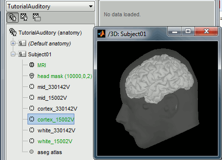
Access the recordings
Link the recordings
- Switch to the "functional data" view.
Right-click on the subject folder > Review raw file
Select the file format: "MEG/EEG: CTF (*.ds...)"
Select all the .ds folders in: sample_auditory/data
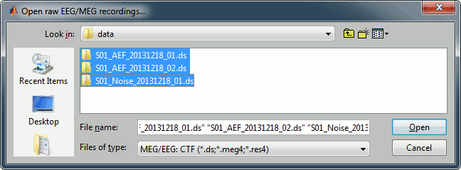
Refine registration now? YES
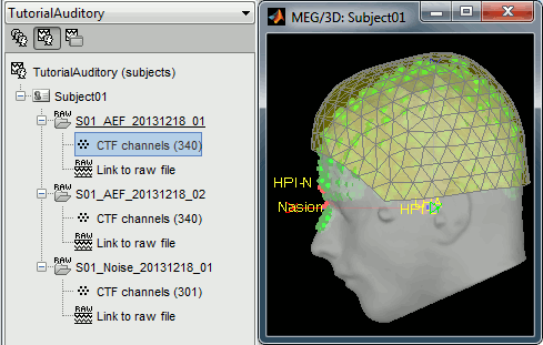
Multiple runs and head position
The two AEF runs 01 and 02 were acquired successively, the position of the subject's head in the MEG helmet was estimated twice, once at the beginning of each run. The subject might have moved between the two runs. To evaluate visually the displacement between the two runs, select at the same time all the channel files you want to compare (the ones for run 01 and 02), right-click > Display sensors > MEG.
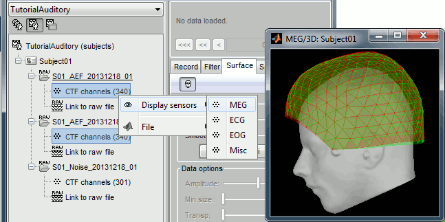
- Typically, we would like to group the trials coming from multiple runs by experimental conditions. However, because of the subject's movements between runs, it's not possible to directly compare the sensor values between runs because they probably do not capture the brain activity coming from the same regions of the brain.
- You have three options if you consider grouping information from multiple runs:
Method 1: Process all the runs separately and average between runs at the source level: The more accurate option, but requires a lot more work, computation time and storage.
Method 2: Ignore movements between runs: This can be acceptable for commodity if the displacements are really minimal, less accurate but much faster to process and easier to manipulate.
Method 3: Co-register properly the runs using the process Standardize > Co-register MEG runs: Can be a good option for displacements under 2cm. Warning: This method has not be been fully evaluated on our side, to use at your own risk.
- In this tutorial, we will illustrate only method 1: runs are not co-registered.
Epoched vs. continuous
- The CTF MEG system can save two types of files: epoched (.ds) or continuous (_AUX.ds).
- Here we have an intermediate storage type: continuous recordings saved in an "epoched" file. The file is saved as small blocks of recordings of a constant time length (1 second in this case). All those time blocks are contiguous, there is no gap between them.
- Brainstorm can consider this file either as a continuous or an epoched file. By default it imports the regular .ds folders as epoched, but we can change this manually, to process it as a continuous file.
Double-click on the "Link to raw file" for run 01 to view the MEG recordings. You can navigate in the file by blocks of 1s, and switch between blocks using the "Epoch" box in the Record tab. The events listed are relative to the current epoch.
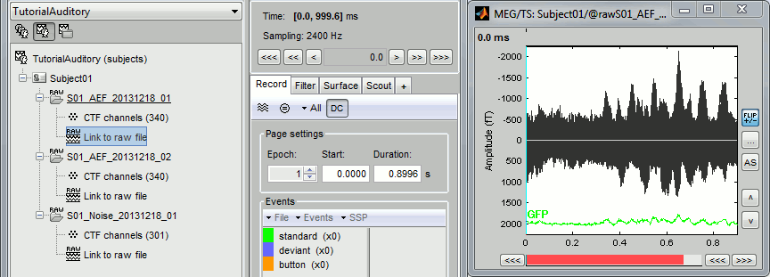
Right-click on the "Link to raw file" for run 01 > Switch epoched/continuous
Double-click on the "Link to raw file" again. Now you can navigate in the file without interruptions. The box "Epoch" is disabled and all the events in the file are displayed at once.
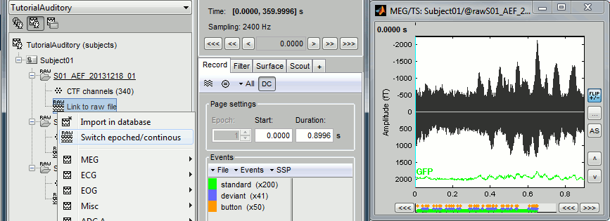
- Repeat this operation twice to convert all the files to a continuous mode.
Run 02 > Switch epoched/continuous
Noise > Switch epoched/continuous
Stimulation markers
Evaluation of the delay
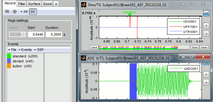
Right-click on Run1/Link to raw file > Stim > Display time series (stimuls channel, UDIO001)
Right-click on Run1/Link to raw file > ADC V > Display time series (audio signal generated, UADC001)
In the Record tab, set the duration of display window to 0.200s.
- Jump to the third event in the "standard" category.
We can observe that there is a delay of about 13ms between the time where the stimulus trigger is generated by the stimulation computer and the moment where the sound is actually played by the sound card of the stimulation computer (delay #1). This is matching the documentation of the experiment in the first section of this tutorial.
Correction of the delay
Delay #1: We can detect the triggers from the analog audio signal (ADC V / UADC001) rather than using the events already detected by the CTF software from the stimulation channel (Stim / UDIO001).
Drag Run01 and Run02 to the Process1 box run "Events > Detect analog triggers":
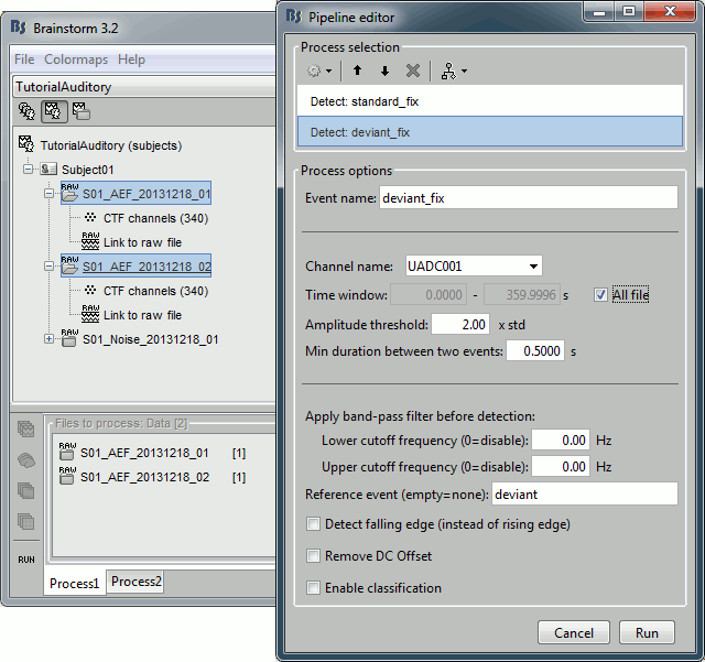
Open Run01 (channel ADC V) to evaluate the correction that was performed by this process. If you look at the third trigger in the "standard" category, you can measure that a 14.6ms correction between event "standard" and the new event "audio".

- There is one more problem to fix: the newly created markers are all called "audio", we lost the classification in "deviant" and "standard". We have now to group the "standard/audio" and "deviant/audio" events.
Keep the two runs selected in Process1 and execute the process "Events > Combine stim/response":
ignore; standard_fix; standard; audio
ignore; deviant_fix; deviant; audio
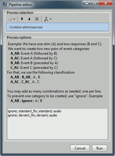
Open Run01 to re-organize the event categories:
Delete the unused event categories: standard, deviant, audio.
Rename standard_fix and deviant_fix to standard and deviant.
Open Run02, delete the unused event categories: standard, deviant, audio
{stim5.gif}Note that we compensated for the jitter delays (delay #1), but not for the other ones (delays #2, #3 and #4). There is still a constant 5ms delay between the stimulus triggers (standard and deviant) and the time where the sound actually reaches the subject's ears.
Detect and remove artifacts
Spectral evaluation
- One of the typical pre-processing steps consist in getting rid of the contamination due to the power lines (50 Hz or 60Hz). Let's start with the spectral evaluation of this file.
Drag ALL the "Link to raw file" to the Process1 box, or easier, just drag the node "Subject01", it will select recursively all the files in it.
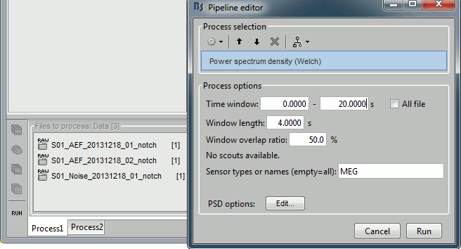
Run the process "Frequency > Power spectrum density (Welch)":
Time window: [0 - 50]s
Window length: 4s
Overlap: 50%
Sensor types or names: MEG
Selected option "Save individual PSD values (for each trial)".
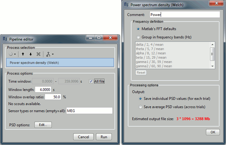
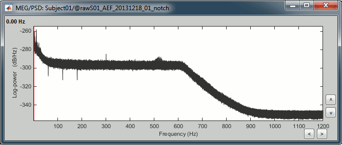
Double-click on the new PSD files to display them.
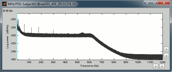
We can observe a series of peaks related with the power lines: 60Hz, 120Hz, 180Hz
(240Hz and 300Hz could be observed as well depending on the window length used for the PSD)The drop after 600Hz corresponds to the low-pass filter applied at the acquisition time.
Power line contamination
Put ALL the "Link to raw file" into the Process1 box (or directly the Subject01 folder)
Run the process: Pre-process > Notch filter
Select the frequencies: 60, 120, 180 Hz
Sensor types or names: MEG
- The higher harmonics are too high to bother us in this analysis, plus they are not clearly visible in all the recordings.
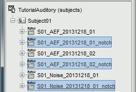
In output, this process creates new .ds folders in the same folder as the original files, and links the new files to the database.
Run again the PSD process "Frequency > Power spectrum density (Welch)" on those new files, with the same parameters, to evaluate the quality of the correction.
Double-click on the new PSD files to open them.
You can zoom in with the mouse wheel to observer what is happening around 60Hz.

To avoid the confusion later, delete the links to the original files: Select the folders containing the original unfiltered files and press the Delete key (or right-click > File > Delete).
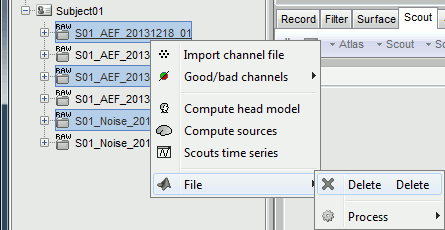
Heartbeats and eye blinks
- Select the two AEF runs in the Process1 box.
- Select successively the following processes, then click on [Run]:
Events > Detect heartbeats: Select channel ECG, check "All file", event name "cardiac".
Events > Detect eye blinks: Select channel VEOG, check "All file", event name "blink".
Events > Remove simultaneous: Remove "cardiac", too close to "blink", delay 250ms.
Compute SSP: Heartbeats: Event name "cardiac", sensor types="MEG", use existing SSP.
Compute SSP: Eyeblinks: Event name "blink", sensor types="MEG", use existing SSP.
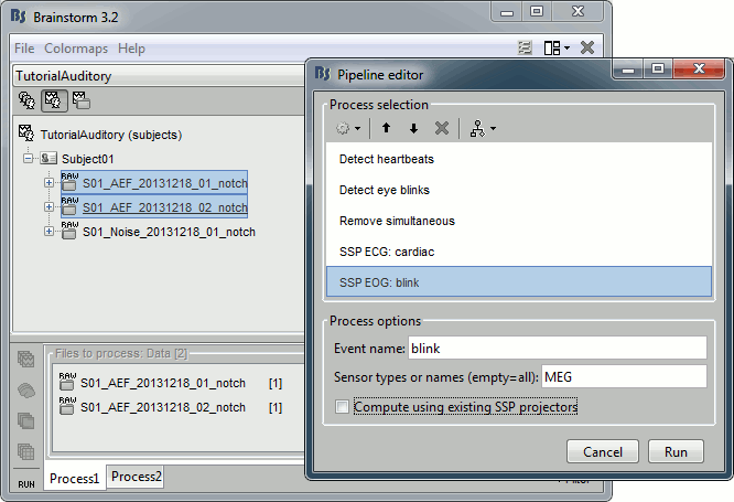
Double-click on Run1 to open the MEG.
Review the EOG and ECG channels and make sure the events detected make sense.
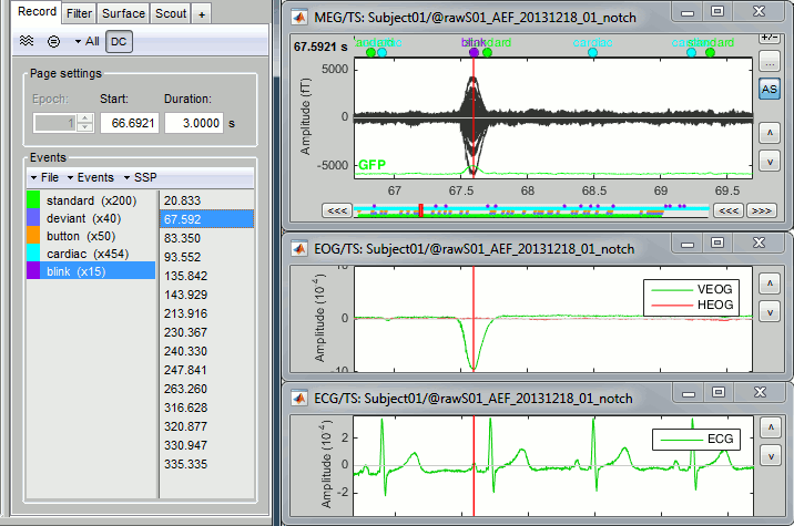
In the Record tab, menu SSP > Select active projectors.
- Blink: The first component is selected and looks good.
- Cardiac: The category is disabled because no component has a value superior to 12%.
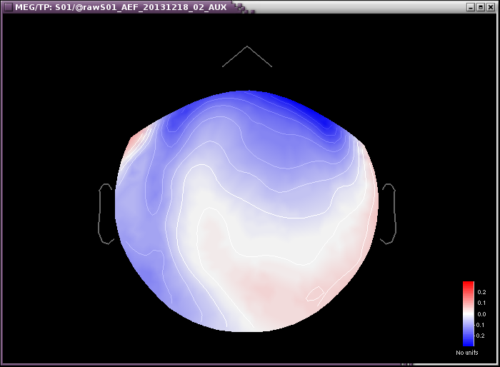
- Select the first component of the cardiac category and display its topography.
It looks exactly like a cardiac topography, keep it selected and click on [Save].

Repeat the same operations for Run2:
- Review the events.
- Select the first cardiac component.
Saccades [TODO]
Run2 contains a few saccades. The automatic detection is not working well.
- Provide an external file of marked saccades to be loaded with this dataset.
- Work on better algorithms for detecting saccades.
Bad segments [TODO]
- Provide a list of bad segments
- Describe the methodology to define those bad segments
Epoching and averaging
Import recordings
To import epochs from Run1:
Right-click on the "Link to raw file" > Import in database
Use events: "standard" and "deviant"
Epoch time: [-100, +500] ms
- Apply the existing SSP (make sure that you have 2 selected projectors)
Remove DC offset based on time window: [-100, 0] ms
UNCHECK the option "Create new conditions for epochs", this way all the epochs are going to be saved in the same Run1 folder, and we will able to separate the trials from Run1 and Run2.
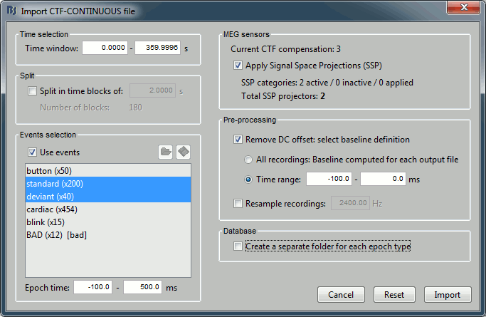
Repeat the same operation for Run2.
Average responses
- As said previously, it is usually not recommended to average recordings in sensor space across multiple acquisition runs because the subject might have moved between the sessions. Different head positions were recorded for each run, we will reconstruct the sources separately for each each run to take into account those movements.
- However, in the case of event-related studies it makes sense to start our data exploration with an average across runs, just to evaluate the quality of the evoked responses. We have seen that the subject almost didn't move between the two runs, so the error would be minimal. We will compute now an approximate sensor average between runs, and we will run a more formal average in source space later.
Drag and drop the two new folders in Process1, run process "Average > Average files"
Select the option "By trial group (subject average)"
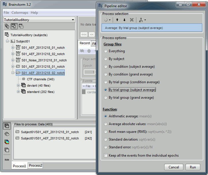
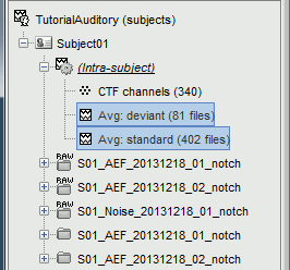
The average for the two conditions "standard" and "deviant" are calculated separately and saved in the folder (intra-subject). The channel file added to this folder is an average of the channel files from Run1 and Run2.
Visual exploration
- Display the two averages, "standard" and "deviant":
Right-click on average > MEG > Display time series
Right-click on average > MISC > Display time series (EEG electrodes Cz and Pz)
Right-click on average > MEG > 2D Sensor cap
In the Filter tab, add a low-pass filter at 150Hz.
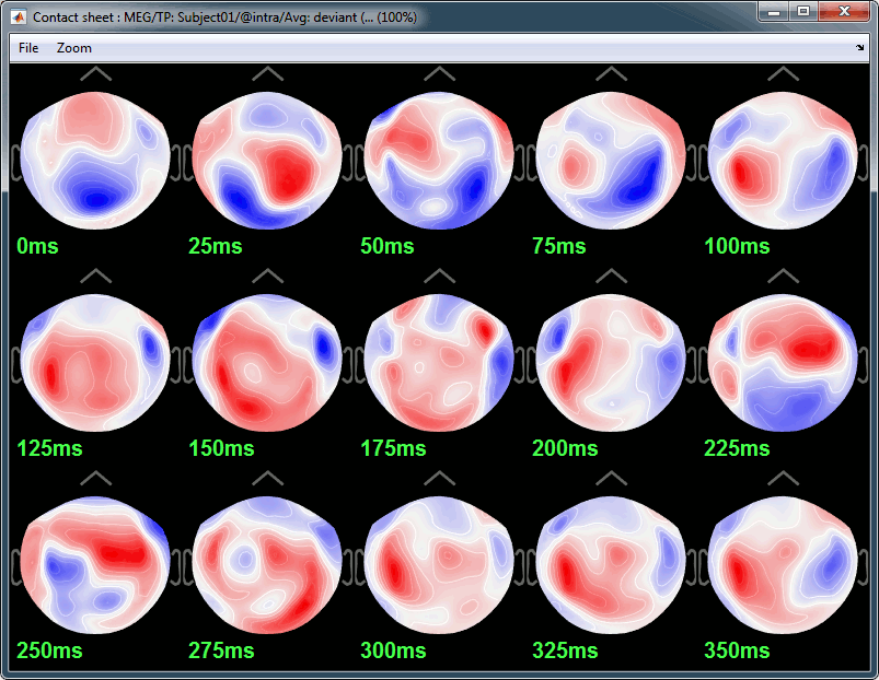
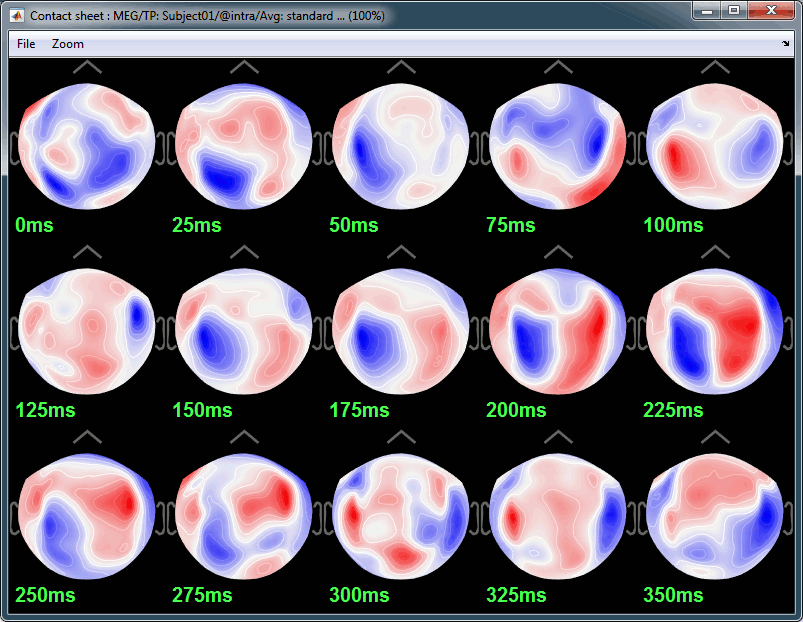
Right-click on the 2D topography figures > Snapshot > Time contact sheet.
Here are results for the standard (top) and deviant (bottom) beeps:
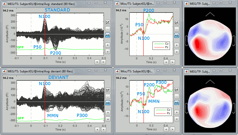
P50: Around 50-60ms, first response in auditory cortex.
N100: Around 100ms, clear auditory response in MEG in both conditions.
P200: Around 185ms, auditory response in both conditions.
P300: Around 300ms, clear component in the EEG for the deviant condition.
Standard:
Deviant:
Source estimation
Head model
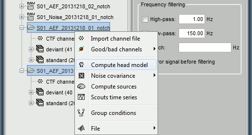
Select the two imported folders at once, right-click > Compute head model
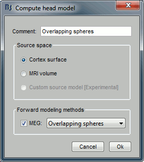
Use the overlapping spheres model and keep all of the options at their default values.
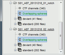
For more information: ?Head model tutorial.
Noise covariance matrix
- We want to calculate the noise covariance from the empty room measurements and use it for the other runs.
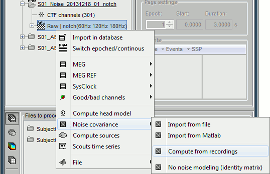
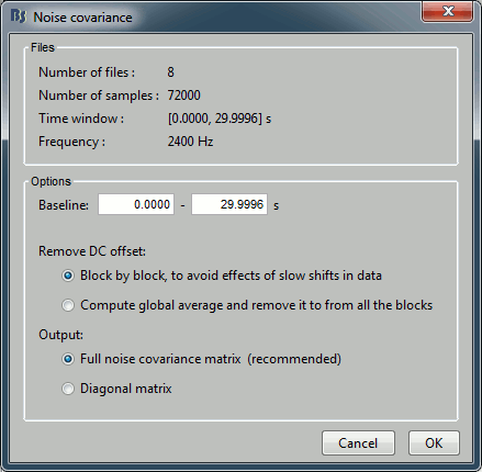
In the Noise folder, right-click on the Link to raw file > Noise covariance > Compute from recordings.
Keep all the default options and click [OK].
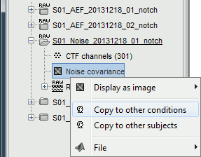
Right-click on the noise covariance file > Copy to other conditions.
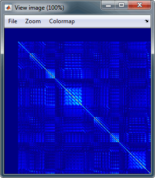
You can double-click on one the copied noise covariance files to check what it looks like:
For more information: ?Noise covariance tutorial.
Inverse model
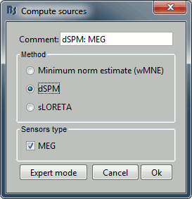
Select the two imported folders at once, right-click > Compute sources
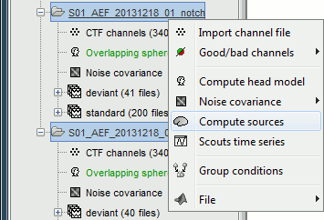
Select minimum norm estimate and keep all the default options.
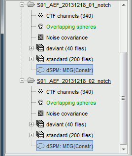
One inverse operator is created in each condition, with one link per data file.
For more information: ?Source estimation tutorial.
Average in source space
- Now we have the source maps available for all the trials, we average them in source space.
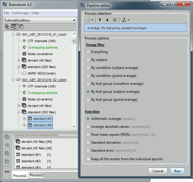
Select the folders for Run1 and Run2 and the [Process sources] button on the left.
Run process "Average > Average files":
Select "By trial group (subject average)"
Double-click on the averages to display them (standard=top, deviant=bottom).
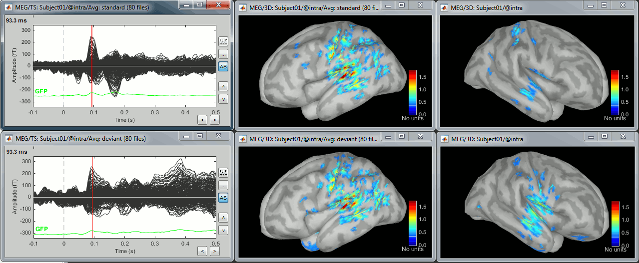
The two conditions have different maximum source values, so the colormap is not scaled in the same way for the two figures by default. To enforce the same scale on the two figures: right-click on one figure > Colormap > Maximum: Custom > 100 pAm.
Z-score noise normalization
- Select the two new averages in Process1.
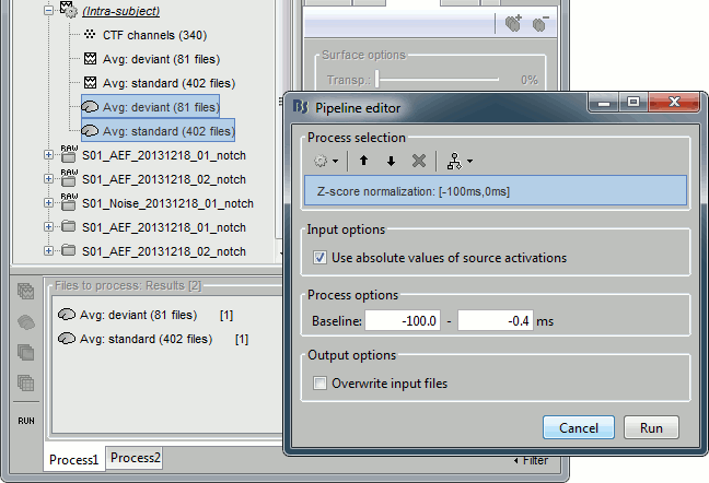
Run process "Standardize > Z-score (dynamic)":
Baseline [-100, -0.4]ms, Use absolue values of source activations
- Double-click on the Z-score files to display them.
Right-click on the figures > Snapshot > Time contact sheet.
ADD 4 CONTACT SHEETS (2 conditions x 2 orientations)
Regions of interest [TODO]
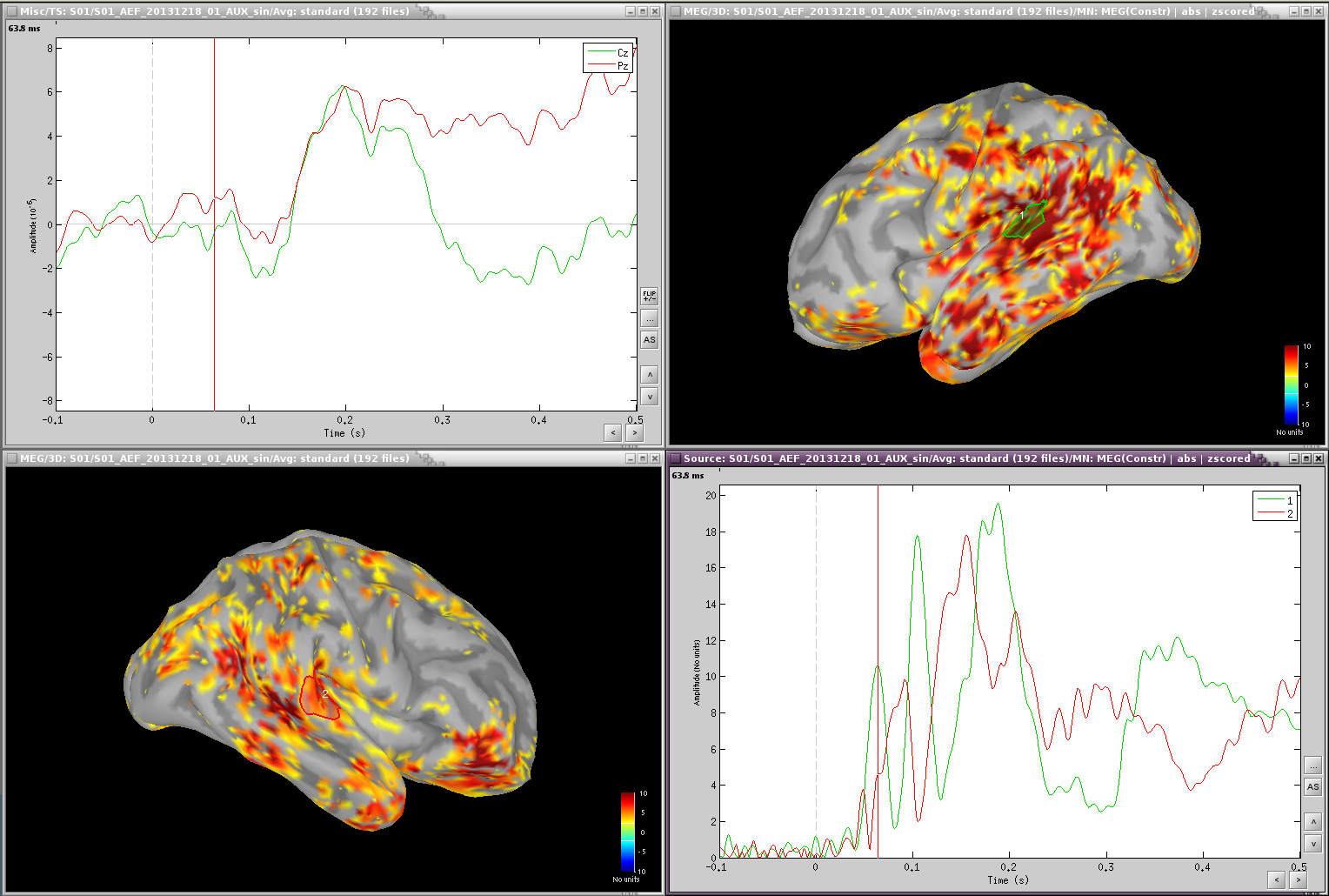
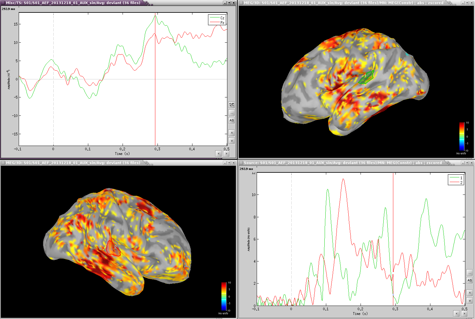
Scouts over primary auditory cortex (A1)
Standard:
Deviant:
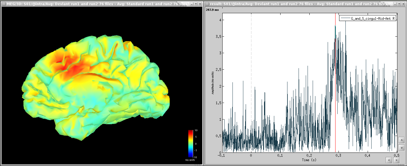
Deviant-standard:
=> Averaged the deviant runs from run1 and run2 (76 trials), then averaged 38 standard trials from run1 with 38 standard trials from run 2 (76 files), subtracted the standard from the deviant and computed sources and z-score.
=> ACC activity around 300ms - this indicates error detection.
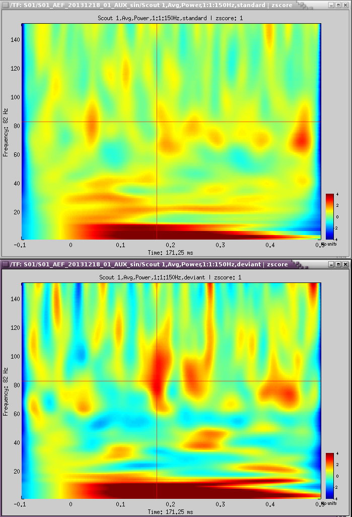
Time-frequency [TODO]
TF over scout 1, z-scored [-100,0] ms
Interesting gamma in the deviant:
Coherence [TODO]
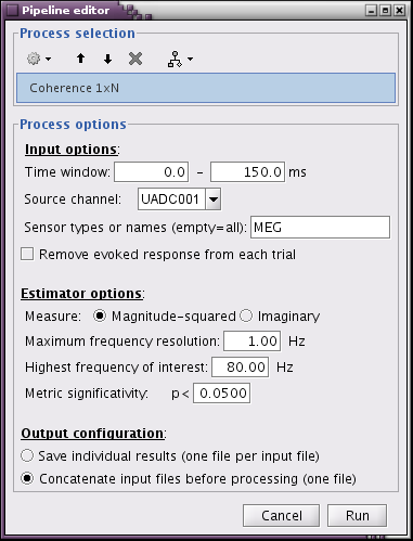
- Run1, sensor magnitude-square coherence 1xN
- UADC001 vs. other sensors
- Time window: [0,150]ms
- Sensor types
- Remove evoked response: NOT SELECTED
- Maximum frequency resolution: 1Hz
- Highest frequency of interest: 80Hz
- Metric significativity: 0.05
- Concatenate input files: SELECTED
=> Coh(0.6Hz,32win)
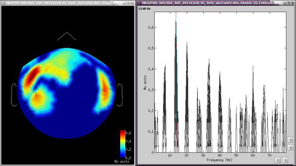
At 13Hz
- Run1, source magnitude-square coherence 1xN
- 50 standard trials
- Highest frequency of interest: 40Hz
Same other inputs
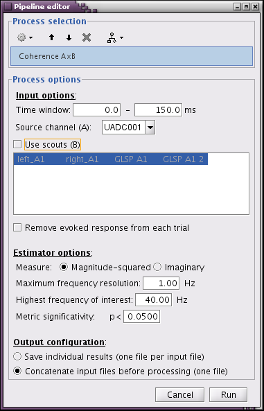
At 13Hz:
![beth_coherence_source_50trials_[0,150]ms_13Hz.png beth_coherence_source_50trials_[0,150]ms_13Hz.png](/brainstorm/Tutorials/Auditory?action=AttachFile&do=get&target=beth_coherence_source_50trials_%5B0%2C150%5Dms_13Hz.png)
Discussion
Discussion about the choice of the dataset on the FieldTrip bug tracker:
http://bugzilla.fcdonders.nl/show_bug.cgi?id=2300
Scripting [TODO]
Process selection
Graphic edition
Generate Matlab script
The operations described in this tutorial can be reproduced from a Matlab script, available in the Brainstorm distribution: brainstorm3/toolbox/script/tutorial_auditory.m
Feedback
