|
Size: 14686
Comment:
|
Size: 18584
Comment:
|
| Deletions are marked like this. | Additions are marked like this. |
| Line 10: | Line 10: |
| == Selecting the trials == We will now compute the average responses for both the "standard" and "deviant" conditions. Two constrains have to be taken into consideration at this stage. |
== Averaging == We will now compute the average responses for both the "standard" and "deviant" conditions. Two constraints have to be taken into consideration at this stage. |
| Line 13: | Line 13: |
| '''Averaging runs separately''': With MEG, it is not recommended to average across acquisition runs with different head positions (ie. different "channel files"). If the head of the subject moved between two blocks of recordings, one sensor does not record the same part of the brain before and after, therefore the runs cannot be compared directly. With EEG, you can generally skip this recommendation. | '''Averaging runs separately''': With MEG, it is not recommended to average sensor data across acquisition runs with different head positions (ie. different "channel files"). If the head of the subject moved between two blocks of recordings, the sensors do not record the same parts of the brain before and after, therefore the runs cannot be compared directly. With EEG, you can generally skip this recommendation. |
| Line 15: | Line 15: |
| '''Using the same number of trials''': As the goal in this analysis is to compare directly the two experimental conditions, we should use the same number of trials for computing the averages. We need to find the group of trials with the lowest number of good trials, and pick the same number in every group. Here we will be limited to 39 trials because of the deviant condition in Run#01. If we had multiple subjects and were planning to compute some group statistics, we should also use equal numbers of trials for all the subjects. The instructions below show how to select easily equal numbers of trials from the database: |
'''Number of trials''': When computing subject-level averages for experimental conditions with different number of trials, you have two options. You can either use the same number of trials for all the conditions and subjects (to make them "more comparable") or use all the available good trials (more samples lead to better estimations of the mean and variance). Here we will go with the second option, using all the trials. See this [[http://neuroimage.usc.edu/brainstorm/Tutorials/Averaging#Number_of_trials|advanced section]] for more details. |
| Line 20: | Line 18: |
| * In the Process1 list, you can notice that the number of imported trials (comment in the database explorer, eg. "40 files") does not match the number of files selected for processing (between brackets, eg. "[39]"). This difference is due to the '''bad trials''' that we have in these folders. The trials tagged with a red dot in the database explorer are ignored by all the processes. The total number of selected files is 468 instead of 480, it means that we have a total of 12 bad trials. * Select the process "'''Files > Select uniform number of trials'''".<<BR>>Select the options: '''By trial group (folder)''' and '''Uniformly distributed'''.<<BR>><<BR>> {{attachment:select_process.gif||height="394",width="532"}} * If you click on [Run], it doesn't do anything but highlighting the first selected file in the database explorer. This process just performs a file selection, it needs to be followed by another one that uses the selected files for computing something. However, you can see what was done in the process report. The reports are displayed only when an error or a warning was reported, but you can open them manually to check for additional messages. Menu '''File > Report viewer'''.<<BR>><<BR>> {{attachment:select_report.gif||height="226",width="633"}} * The comment in the report lists the 4 groups or trials that were identified based on the option we selected (group by trial group and folder), with the maximum number of good trials per group: Run01/deviant (39), Run01/standard (193), Run02/deviant (40), Run01/standard (197).<<BR>>The process picked 39 trials in each group, uniformly distributed in the list of available trials. <<BR>>Example of trial indices select for Run01/standard: [1, 6, 11, 16, 21, 26, 31, 36, ..., 188, 193] |
* In the Process1 box, the number of imported trials (comment in the database explorer, eg. "40 files") does not match the number of files selected for processing (between brackets, eg. "[39]"). This difference is due to the '''bad trials''' that we have in these folders. The trials tagged with a red dot in the database explorer are ignored by all the processes. The total number of selected files is 457 instead of 479, it means that we have a total of 22 bad trials. * Select the process "'''Average > Average files'''".<<BR>>Select the options: '''By trial group (folder)''', Arithmetic average, Keep all the event markers.<<BR>><<BR>> {{attachment:average_folder.gif||height="547",width="525"}} |
| Line 25: | Line 21: |
| == Process options: Select trials == Available options in the process: File > Select uniform number of trials. * '''By folder''': Groups by subject and by folder, ignoring the trial groups. <<BR>>In the current configuration, it would produce two files, one for each acquisition run. * '''By trial group (folder)''': Groups by set of trials with the same name, separately for each folder and each subject. * '''By trial group (subject)''': Groups by set of trials with the same name, for each subject. The separation in folders is ignored. In the current configuration, it would produce two files, one for "deviant" and one for "standard". How to select trials in a group that contains more than the requested number (Nf files, selecting only Ns): * '''Random selection''': Select a random subset of Ns trials, using randperm(Nf,Ns). * '''First in the list''': Select the first Ns trials (trial indices: 1:Ns). * '''Last in the list''': Select the last Ns trials (trial indices: Nf-Ns+1:Nf). * '''Unformly distributed''': Select Ns equally spaced trials (trial indices: round(linspace(1, Nf, Ns))). == Averaging == * Reload last process executed with the menu: '''File > Reload last pipeline'''. * Add the process "'''Average > Average files'''" after trial selection process. <<BR>>Select the options: By trial group (folder average), Arithmetic average, Keep all the event markers.<<BR>><<BR>> {{attachment:average_folder.gif||height="576",width="561"}} * You get two new files for each average, each one computed from 39 trials: <<BR>><<BR>> {{attachment:average_files.gif||height="223",width="247"}} |
* You get two new files for each acquisition run. The number between parenthesis indicates how many good trials were used to compute each average. <<BR>><<BR>> {{attachment:average_files.gif||height="229",width="250"}} |
| Line 45: | Line 24: |
| Description of all the options of the process: | Description of all the options of the process: Average > Average files. |
| Line 51: | Line 30: |
| * '''By trial group (folder average)''': Groups by set of trials with the same name, separately for each folder and each subject. * '''By trial group (subject average)''': Groups by set of trials with the same name, for each subject. The separation in folders is ignored. In the current configuration, it would produce two files, one for "deviant" and one for "standard". |
* '''By trial group (folder average)''': Groups by set of trials with the same name, separately for each folder and each subject. Here it creates four groups (two folders x two trial groups). * '''By trial group (subject average)''': Groups by set of trials with the same name, for each subject. The separation in folders is ignored. Here it would produce two files (deviant and standard). |
| Line 55: | Line 34: |
| * '''Weighted average''': When averaging single trials, the number of files is saved in the field nAvg of the average file. When re-averaging the averages across acquisition sessions or subjects, this field nAvg can be used to weigh each file with the number of trials from which it was computed: <<BR>>mean(x) = sum(nAvg(i) * x(i)) / sum(nAvg(i))<<BR>>In most cases, this option should be selected when averaging within a subject and disabled when averaging across subjects. It has no impact in the current example (no averages, nAvg=1). | |
| Line 58: | Line 38: |
| The average response contains interesting information about the brain operations that occur shortly after the presentation of the stimulus. We can explore two dimensions: the '''location''' of the various brain regions involved in the sensory processing and the precise '''timing''' of their activation. Because these two types of information are of equal interest, we typically explore the recordings with two figures at the same time, one that shows all the signals in time, one that shows the spatial distribution at one instant. | The average response contains interesting information about the brain operations that occur shortly after the presentation of the stimulus. We can explore two dimensions: the '''location''' of the various brain regions involved in the sensory processing and the precise '''timing''' of their activation. Because these two types of information are of equal interest, we typically explore the recordings with two figures at the same time, one that shows all the signals in time and one that shows their spatial distribution at one instant. |
| Line 62: | Line 42: |
| * In the Filter tab: Add a '''low-pass filter''' at '''100Hz'''. | * In the Filter tab: Add a '''low-pass filter''' at '''40Hz'''. |
| Line 74: | Line 54: |
| * Open the "standard" average in the same way and delete the "cardiac" markers. | |
| Line 77: | Line 58: |
| * Open the MEG recordings. * Delete the "cardiac" markers. * The average is cleaner because it was computed from many more trials, but it also contains more unwanted things: a few blinks and probably an error from the subject. The "button" marker at 136ms is not supposed to be here. The task is so easy that we can probably assume that it is not a real detection error but rather a manipulation error, therefore it should not affect the cortical response in the very early stages of the stimulus processing, which is what we are exploring now. |
* Open the MEG recordings for deviant and standard. * Delete the "cardiac" markers in both files. |
| Line 89: | Line 69: |
| * In the Filter tab: add a '''low-pass filter''' at '''100Hz'''. | * In the Filter tab: add a '''low-pass filter''' at '''40Hz''' (it makes the figures easier to read). |
| Line 91: | Line 71: |
| * Here are the results for the standard (top) and deviant (bottom) beeps: <<BR>><<BR>> {{attachment:average_summary.gif||height="371",width="663"}} | * Here are the results for the standard (top) and deviant (bottom) beeps: <<BR>><<BR>> {{attachment:average_summary.gif||width="650"}} |
| Line 100: | Line 80: |
| * Some seem to have a direct correspondance in MEG (N100) some don't (P300). | * Some seem to have a direct correspondence in MEG (N100) some don't (P300). Additional quality check with the event markers: * The standard average shows two unwanted events between 100ms and 200ms post-stimulus, one "blink" and one "button" response. The trials that contain them should be marked as bad and the average recomputed, because the subject is probably not doing the task correctly. * We will not do this here because the SNR is high enough anyway, but remember that this option "Keep all events" from the averaging process provides a good summary of the recordings and can help you identify some bad trials. <<TAG(Advanced)>> == Averaging bad channels == The bad channels can be defined independently for each trial, therefore we can have different numbers of data points averaged for different electrodes. If we have a channel A considered good for N<<HTML(<SUB>A</SUB>)>> trials, the corresponding channel in the average file is computed in this way: sum(N<<HTML(<SUB>A</SUB>)>> trials) / N<<HTML(<SUB>A</SUB>)>>. In the average file, a channel is considered good if it is good in at least one trial, and considered as bad if it is bad in all the trials. The entire file is then considered as if it were computed from the maximum number of good trials: N<<HTML(<SUB>max</SUB>)>> = max(N<<HTML(<SUB>i</SUB>)>>), i=1..N<<HTML(<SUB>trials</SUB>)>>. This procedure allows the conservation of the maximum amount of data. However it may cause some unwanted effects across channels: the SNR might be higher for some channels than others. If you want to avoid this: mark the channels as bad in all the trials, or report all the bad channels to the average file. This can be done easily using the database explorer, see tutorial [[Tutorials/BadChannels|Bad channels]]. |
| Line 105: | Line 99: |
| As said previously, it is usually not recommended to average recordings in sensor space across multiple acquisition runs because the subject might have moved between the sessions. Different head positions were recorded for each run, we will reconstruct the sources separately for each each run to take into account these movements. | As said previously, it is usually not recommended to average MEG recordings in sensor space across multiple acquisition runs because the subject might have moved between the sessions. Different head positions were recorded for each run, so we will reconstruct the sources separately for each each run to take into account these movements. |
| Line 113: | Line 107: |
| * To run again the same process with different parameters: '''File > Reload last pipeline'''. Select: * '''By trial group (subject average)''': It will compute one average per experimental condition. * '''Arithmetic average + Standard error''': It will save in the same file the average and the standard error across all the trials. Illustrated in the next section. |
* To run the same process again with different parameters: '''File > Reload last pipeline'''. Select: * '''By trial group (subject average)''': One average per experimental condition, across acquisition runs * '''Arithmetic average + Standard error''': Save the standard error across all the trials in the same file |
| Line 117: | Line 111: |
| * The two files that are created are now saved in a new folder "'''Intra-subject'''". This is where all the results of processes involving multiple folders within one subject will be saved.<<BR>><<BR>> {{attachment:average_stderror.gif||height="184",width="219"}} | * The two averages are saved in the folder "'''Intra-subject'''". This is where all the results of processes involving multiple folders, within one subject, will be saved.<<BR>><<BR>> {{attachment:average_stderror.gif||height="184",width="219"}} * Delete these files to avoid any confusion later. |
| Line 122: | Line 117: |
| If you computed the '''standard deviation''' or the '''standard deviation''' together with an average, it will be automatically represented in the time series figures. | If you computed the '''standard deviation''' or the '''standard error''' together with an average, it will be automatically represented in the time series figures. |
| Line 126: | Line 121: |
| * Select two sensors and plot them separately (right-click > Channels > View selected, or "Enter").<<BR>>The green and red areas represent at each time point the standard error around the signal.<<BR>><<BR>> {{attachment:stderror.gif||height="176",width="379"}} | * Select two sensors and plot them separately (right-click > Channels > View selected, or "Enter").<<BR>>The green and red areas represent, at each time point, the standard error around the signal.<<BR>><<BR>> {{attachment:stderror.gif||height="176",width="379"}} |
| Line 128: | Line 123: |
| * Right-click on the file > '''File > View file contents'''. <<BR>>The average is saved in the field '''F''', the standard error is saved in the field '''Std'''.<<BR>><<BR>> {{attachment:stderror_file.gif||height="230",width="396"}} | <<TAG(Advanced)>> == Number of trials == You should always be careful when comparing averages computed from different numbers of trials. In most cases, you can safely include '''all the trials''' in your averages, even in the case of imbalanced designs. However, for very low numbers of trials or when comparing peak amplitudes, having the same number of trials becomes more critical. See the following references for more details: * Luck SJ (2010)<<BR>>[[http://erpinfo.org/educational-materials/comments-on-comparing-conditions-with-different-numbers-of-trials-1|Is it Legitimate to Compare Conditions with Different Numbers of Trials?]] * Thomas DG, Grice JW, Najm-Briscoe RG, Miller JW (2004)<<BR>>[[http://www.ncbi.nlm.nih.gov/pubmed/15525568|The influence of unequal numbers of trials on comparisons of average event-related potentials]] <<TAG(Advanced)>> == Selecting equal numbers of trials == If you decided you want to use the same number of trials across all the experimental conditions and/or across all the subjects, you can use a process to select them easily from the database. * Drag and drop all the "'''standard'''" and "'''deviant'''" trials for '''both runs''' in Process1. * Select the process "'''Files > Select uniform number of trials'''".<<BR>>Select the options: '''By trial group (folder)''' and '''Uniformly distributed'''.<<BR>><<BR>> {{attachment:select_process.gif||height="494",width="483"}} * If you click on [Run], it doesn't do anything but highlighting the first selected file in the database explorer. This process just performs a file selection, it needs to be followed by another process that uses the selected files for computing something. However, you can see what was done in the process report. The reports are displayed only when an error or a warning was reported, but you can open them manually to check for additional messages. Menu '''File > Report viewer'''.<<BR>><<BR>> {{attachment:select_report.gif||height="235",width="666"}} * The comment in the report shows the 4 groups of trials that were identified based on the option we selected (group "by trial group and folder"), with the number of good trials per group. <<BR>>The process picked 39 trials in each group, uniformly distributed in the list of available trials. <<BR>>Example of trial indices selected for Run01/standard: [1, 6, 11, 16, 21, 26, 31, 36, ..., 188, 193] * To average these selected trials together, you would just need to add the process "Average > Average files" after this selection process in the pipeline editor. <<BR>><<BR>> {{attachment:average_selected.gif||height="168",width="374"}} ==== Process options ==== Available options in the process: File > Select uniform number of trials. * '''By folder''': Groups by subject and by folder, ignoring the trial groups. <<BR>>Here, it would identify two groups, one for each acquisition run: Run01, Run02. * '''By trial group (folder)''': Groups by set of trials with the same name, separately for each folder and each subject. Here it would identify four groups: Run01/deviant, Run01/standard, Run02/deviant, Run01/standard. * '''By trial group (subject)''': Groups by set of trials with the same name, for each subject. The separation in folders is ignored. Here it would identify two groups: deviant, standard. How many trials to select in each group: * '''Number of trials per group''': This number of trials must be available in all the groups. If set to 0, the group with the lowest number of good trials is identified and the same number of trials is selected from all the other groups. How to select trials in a group that contains more than the requested number (Nf files, selecting only Ns): * '''Random selection''': Select a random subset of Ns trials. Trial indices: randperm(Nf,Ns) * '''First in the list''': Select the first Ns trials. Trial indices: 1:Ns * '''Last in the list''': Select the last Ns trials. Trial indices: Nf-Ns+1:Nf * '''Uniformly distributed''': Select Ns equally spaced trials. Trial indices: round(linspace(1, Nf, Ns))) == On the hard drive == The average files have the same structure as the individual trials, described in the tutorial [[http://neuroimage.usc.edu/brainstorm/Tutorials/Epoching#On_the_hard_drive|Import epochs]]. . {{attachment:average_struct.gif||height="335",width="536"}} '''Differences with the imported epochs''' * '''F''': [Nchannels x Ntime] average recordings across all the trials, in Volts. * '''Std''': [Nchannels x Ntime] standard error or standard deviation across all the trials, in Volts. * '''nAvg''': Number of good trials that were used to compute the average. |
Tutorial 16: Average response
Authors: Francois Tadel, Elizabeth Bock, Sylvain Baillet
All the epochs we have imported in the previous tutorial are represented by matrices that have the same size (same number of channels, same number of time points), therefore they can be averaged together by experimental condition. The result is called indifferently "evoked response", "average response", "event-related field" in MEG (ERF) or "event-related potential" in EEG (ERP). It shows the components of the brain signals that are strictly time-locked to the presentation of a stimulus.
Contents
Averaging
We will now compute the average responses for both the "standard" and "deviant" conditions. Two constraints have to be taken into consideration at this stage.
Averaging runs separately: With MEG, it is not recommended to average sensor data across acquisition runs with different head positions (ie. different "channel files"). If the head of the subject moved between two blocks of recordings, the sensors do not record the same parts of the brain before and after, therefore the runs cannot be compared directly. With EEG, you can generally skip this recommendation.
Number of trials: When computing subject-level averages for experimental conditions with different number of trials, you have two options. You can either use the same number of trials for all the conditions and subjects (to make them "more comparable") or use all the available good trials (more samples lead to better estimations of the mean and variance). Here we will go with the second option, using all the trials. See this advanced section for more details.
Drag and drop all the "standard" and "deviant" trials for both runs in Process1.
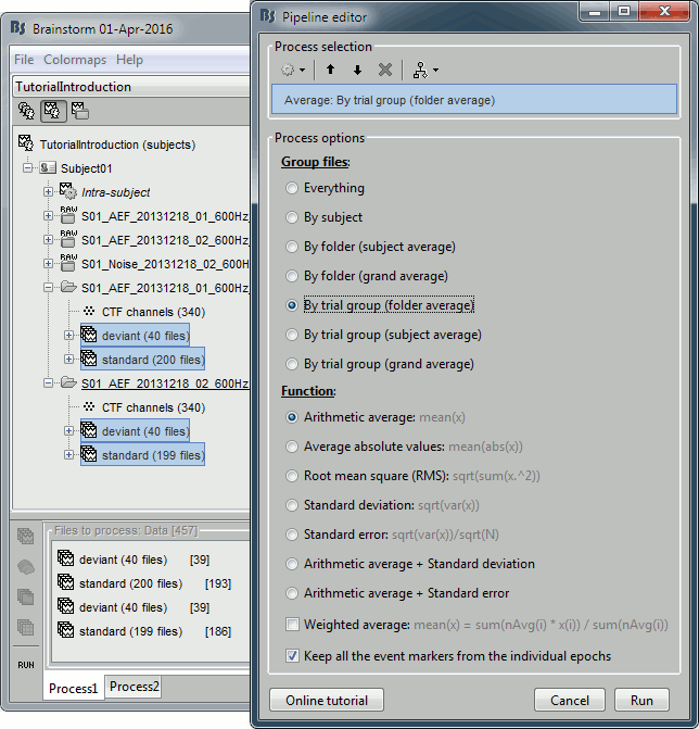
In the Process1 box, the number of imported trials (comment in the database explorer, eg. "40 files") does not match the number of files selected for processing (between brackets, eg. "[39]"). This difference is due to the bad trials that we have in these folders. The trials tagged with a red dot in the database explorer are ignored by all the processes. The total number of selected files is 457 instead of 479, it means that we have a total of 22 bad trials.
Select the process "Average > Average files".
Select the options: By trial group (folder), Arithmetic average, Keep all the event markers.
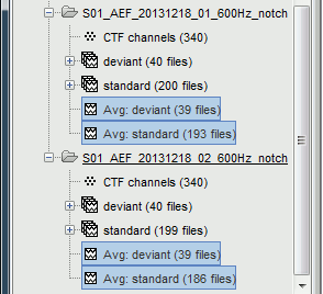
You get two new files for each acquisition run. The number between parenthesis indicates how many good trials were used to compute each average.
Process options: Average
Description of all the options of the process: Average > Average files.
Everything: Averages all the files selected in Process1 together, creates only one file in output.
By subject: Groups the files by subject (ignoring the folders), creates one file per subject.
By folder (subject average): Groups by subject and by folder, ignoring the trial groups.
In the current configuration, it would produce two files, one for each acquisition run.By folder (grand average): Groups by folder, across the subjects. All the files located in folders with the same name would be averaged together, no matter in what subject they are.
By trial group (folder average): Groups by set of trials with the same name, separately for each folder and each subject. Here it creates four groups (two folders x two trial groups).
By trial group (subject average): Groups by set of trials with the same name, for each subject. The separation in folders is ignored. Here it would produce two files (deviant and standard).
By trial group (grand average): Groups by set of trials with the same name, ignoring the classification by folder or subject.
Function: Documented directly in the option panel.
Weighted average: When averaging single trials, the number of files is saved in the field nAvg of the average file. When re-averaging the averages across acquisition sessions or subjects, this field nAvg can be used to weigh each file with the number of trials from which it was computed:
mean(x) = sum(nAvg(i) * x(i)) / sum(nAvg(i))
In most cases, this option should be selected when averaging within a subject and disabled when averaging across subjects. It has no impact in the current example (no averages, nAvg=1).Keep all the event markers: If this option is selected, all the event markers that were available in all the individual trials are reported to the average file. It can be useful to check the relative position of the artifacts or the subject responses, or quickly detect some unwanted configuration such as a subject who would constantly blink immediately after a visual stimulus.
Visual exploration
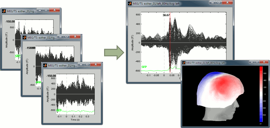
The average response contains interesting information about the brain operations that occur shortly after the presentation of the stimulus. We can explore two dimensions: the location of the various brain regions involved in the sensory processing and the precise timing of their activation. Because these two types of information are of equal interest, we typically explore the recordings with two figures at the same time, one that shows all the signals in time and one that shows their spatial distribution at one instant.
Open the MEG recordings for the deviant average in Run#01: double-click on the file.
- In the Record tab: Select the "butterfly" view more (first button in the toolbar).
In the Filter tab: Add a low-pass filter at 40Hz.
In the Record tab: Delete the "cardiac" event type, we are not interested by their distribution.

This figure shows a typical clean evoked response, with a high signal-to-noise ratio. This represents the brain response to a simple auditory stimulation, the large peak around 90ms probably corresponds to the main response in the primary auditory cortex.
The green line represents the global field power (GFP), ie the sum of the square of all the sensors at each time point. This measure is sometimes used to identify transient or stable states in ERP/ERF.
- This is the response to the deviant beeps (clearly higher in pitch), for which the subject is supposed to press a button to indicate that he/she detected the target. These responses are represented with the "button" events, distributed between 350ms and the end of the file (many responses happened after 500ms). Because of the variability in the response times, we can already anticipate that we won't be able to study correctly the motor response from this average. For studying the activity in the motor area, we need to epoch the recordings again around the "button" events.
Add a spatial view:
Open a 2D topography for the same file (right-click on the figure > View topography, or Ctrl+T).
Review the average as a movie with the keyboard shortcuts (hold the left or right arrow key).
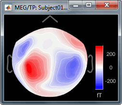
At 90ms, we can observe a typical topography for a bilateral auditory response. Both on the left sensors and the right sensors we observe field patterns which seem to indicate a dipolar-like activity in the temporal or central regions.
Close everything with the button [X] in the top-right corner of the Brainstorm window.
Accept to save the modifications (you deleted the "cardiac" events).- Open the "standard" average in the same way and delete the "cardiac" markers.
Repeat the same operations for Run#02:
- Open the MEG recordings for deviant and standard.
- Delete the "cardiac" markers in both files.
- Open a 2D topography and review the recordings.
- Close everything.
Interpretation
Let's display the two conditions "standard" and "deviant" side-by-side, for Run#01.
Right-click on average > MEG > Display time series.
Right-click on average > MISC > Display time series (EEG electrodes Cz and Pz)
Right-click on average > MEG > 2D Sensor cap
In the Filter tab: add a low-pass filter at 40Hz (it makes the figures easier to read).
In the Record tab: you can set a common amplitude scale for all the figures with the button [=].
Here are the results for the standard (top) and deviant (bottom) beeps:
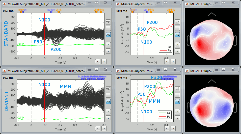
The legend in blue shows names often used in the EEG ERP literature:
P50: 50ms, bilateral auditory response in both conditions.
N100: 95ms, bilateral auditory response in both conditions.
MMN: 230ms, mismatch negativity in the deviant condition only (detection of an abnormality).
P200: 170ms, in both conditions but much stronger in the standard condition.
P300: 300ms, deviant condition only (decision making in preparation of the button press).
- Some seem to have a direct correspondence in MEG (N100) some don't (P300).
Additional quality check with the event markers:
- The standard average shows two unwanted events between 100ms and 200ms post-stimulus, one "blink" and one "button" response. The trials that contain them should be marked as bad and the average recomputed, because the subject is probably not doing the task correctly.
- We will not do this here because the SNR is high enough anyway, but remember that this option "Keep all events" from the averaging process provides a good summary of the recordings and can help you identify some bad trials.
Averaging bad channels
The bad channels can be defined independently for each trial, therefore we can have different numbers of data points averaged for different electrodes. If we have a channel A considered good for NA trials, the corresponding channel in the average file is computed in this way: sum(NA trials) / NA.
In the average file, a channel is considered good if it is good in at least one trial, and considered as bad if it is bad in all the trials. The entire file is then considered as if it were computed from the maximum number of good trials: Nmax = max(Ni), i=1..Ntrials.
This procedure allows the conservation of the maximum amount of data. However it may cause some unwanted effects across channels: the SNR might be higher for some channels than others. If you want to avoid this: mark the channels as bad in all the trials, or report all the bad channels to the average file. This can be done easily using the database explorer, see tutorial Bad channels.
Averaging across runs
As said previously, it is usually not recommended to average MEG recordings in sensor space across multiple acquisition runs because the subject might have moved between the sessions. Different head positions were recorded for each run, so we will reconstruct the sources separately for each each run to take into account these movements.
However, in the case of event-related studies it makes sense to start our data exploration with an average across runs, just to evaluate the quality of the evoked responses. We have seen in tutorial #4 that the subject almost didn't move between the two runs, so the error would be minimal.
Let's compute an approximate average across runs. We will run a formal average in source space later.
To run the same process again with different parameters: File > Reload last pipeline. Select:
By trial group (subject average): One average per experimental condition, across acquisition runs
Arithmetic average + Standard error: Save the standard error across all the trials in the same file
Keep all the event markers: Do not select this option, we've already seen what it does.
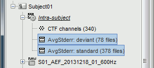
The two averages are saved in the folder "Intra-subject". This is where all the results of processes involving multiple folders, within one subject, will be saved.
- Delete these files to avoid any confusion later.
Standard error
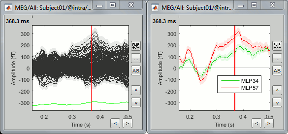
If you computed the standard deviation or the standard error together with an average, it will be automatically represented in the time series figures.
Double-click on one of the AvgStderr files to display the MEG sensors.
The light-grey area around the sensors represent the maximum standard error around the maximum and minimum values across all the sensors.Select two sensors and plot them separately (right-click > Channels > View selected, or "Enter").
The green and red areas represent, at each time point, the standard error around the signal.
Number of trials
You should always be careful when comparing averages computed from different numbers of trials. In most cases, you can safely include all the trials in your averages, even in the case of imbalanced designs. However, for very low numbers of trials or when comparing peak amplitudes, having the same number of trials becomes more critical. See the following references for more details:
Luck SJ (2010)
Is it Legitimate to Compare Conditions with Different Numbers of Trials?Thomas DG, Grice JW, Najm-Briscoe RG, Miller JW (2004)
The influence of unequal numbers of trials on comparisons of average event-related potentials
Selecting equal numbers of trials
If you decided you want to use the same number of trials across all the experimental conditions and/or across all the subjects, you can use a process to select them easily from the database.
Drag and drop all the "standard" and "deviant" trials for both runs in Process1.
Select the process "Files > Select uniform number of trials".
Select the options: By trial group (folder) and Uniformly distributed.
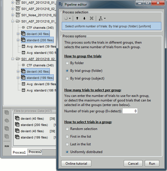
If you click on [Run], it doesn't do anything but highlighting the first selected file in the database explorer. This process just performs a file selection, it needs to be followed by another process that uses the selected files for computing something. However, you can see what was done in the process report. The reports are displayed only when an error or a warning was reported, but you can open them manually to check for additional messages. Menu File > Report viewer.
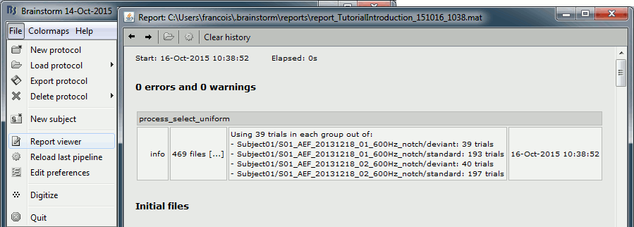
The comment in the report shows the 4 groups of trials that were identified based on the option we selected (group "by trial group and folder"), with the number of good trials per group.
The process picked 39 trials in each group, uniformly distributed in the list of available trials.
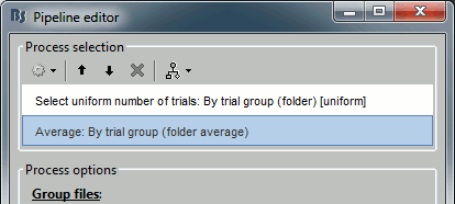
Example of trial indices selected for Run01/standard: [1, 6, 11, 16, 21, 26, 31, 36, ..., 188, 193]To average these selected trials together, you would just need to add the process "Average > Average files" after this selection process in the pipeline editor.
Process options
Available options in the process: File > Select uniform number of trials.
By folder: Groups by subject and by folder, ignoring the trial groups.
Here, it would identify two groups, one for each acquisition run: Run01, Run02.By trial group (folder): Groups by set of trials with the same name, separately for each folder and each subject. Here it would identify four groups: Run01/deviant, Run01/standard, Run02/deviant, Run01/standard.
By trial group (subject): Groups by set of trials with the same name, for each subject. The separation in folders is ignored. Here it would identify two groups: deviant, standard.
How many trials to select in each group:
Number of trials per group: This number of trials must be available in all the groups. If set to 0, the group with the lowest number of good trials is identified and the same number of trials is selected from all the other groups.
How to select trials in a group that contains more than the requested number (Nf files, selecting only Ns):
Random selection: Select a random subset of Ns trials. Trial indices: randperm(Nf,Ns)
First in the list: Select the first Ns trials. Trial indices: 1:Ns
Last in the list: Select the last Ns trials. Trial indices: Nf-Ns+1:Nf
Uniformly distributed: Select Ns equally spaced trials. Trial indices: round(linspace(1, Nf, Ns)))
On the hard drive
The average files have the same structure as the individual trials, described in the tutorial Import epochs.
Differences with the imported epochs
F: [Nchannels x Ntime] average recordings across all the trials, in Volts.
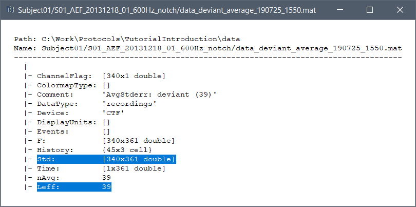
Std: [Nchannels x Ntime] standard error or standard deviation across all the trials, in Volts.
nAvg: Number of good trials that were used to compute the average.

