|
Size: 7984
Comment:
|
Size: 8501
Comment:
|
| Deletions are marked like this. | Additions are marked like this. |
| Line 4: | Line 4: |
| It is common during the acquisition to have a few sensors that are recording values that will not be usable in the data analysis. In MEG, a sensor can be damaged or unstable. In EEG, the quality of the connection between the electrode and the subject scalp is sometimes too low to record anything interesting. | It is common during the acquisition to have a few sensors that are recording values that will not be usable in the data analysis. In MEG, a sensor can be damaged or unstable. In EEG, the quality of the connection between the electrode and the scalp is sometimes too low to record anything interesting. |
| Line 15: | Line 15: |
| Some bad channels are easy to detect, their signals look either completely off or totally flat compared with the other surrounding sensors. Some others are more difficult to identify. You may be able to observe that something looks wrong in various ways (the examples below are taken from other datasets): | Some bad channels are easy to detect, their signals look either completely off or totally flat compared with the other surrounding sensors. Some others are more difficult to identify. The examples below are taken from other datasets. |
| Line 17: | Line 17: |
| * In the PSD file we always recommend to compute for all the datasets (power spectrum density): <<BR>><<BR>> {{attachment:psd_neck.gif||height="146",width="423"}} {{attachment:bad_psd.gif||height="140",width="213"}} * Simply looking at the signals traces, if some channels appear generally noisier than the others: <<BR>><<BR>> {{attachment:bad_signal.gif||height="122",width="266"}} * Looking at a 2D sensor topography, if one sensor always has different values from its neighbors: <<BR>><<BR>> {{attachment:bad_topo.gif}} * In the source maps, if you see only one region of the cortex activated all the time. |
* The power spectrum density (PSD) is usually a good way to spot a few bad channels, this is why we always recommend to compute it for all the datasets:<<BR>><<BR>> {{attachment:psd_neck.gif||height="146",width="423"}} {{attachment:bad_psd.gif||height="140",width="213"}} {{attachment:psd_neck_ncm.png||height="146",width="423"}} {{attachment:bad_psd.gif||height="140",width="213"}} * Simply looking at the signals traces, some channels may appear generally noisier than the others: <<BR>><<BR>> {{attachment:bad_signal.gif||height="122",width="266"}} * Looking at a 2D sensor topography, if one sensor shows very different values from its neighbors for extended periods of time, you can doubt of its quality: <<BR>><<BR>> {{attachment:bad_topo.gif||height="128",width="335"}} |
| Line 25: | Line 25: |
| * Double-click on the recordings for run #01 to open the MEG sensors.<<BR>>Select only one subset of sensor (in the drop-down menu in the Record tab, eg. "CTF LT"). | * Double-click on the recordings for run #01 to open the MEG sensors. |
| Line 28: | Line 28: |
| * If you can't see anything because the topography figure is too small, you can change the way the figures are arranged automatically. In the top-right corner of the Brainstorm figure, select the menu "Window layout options > Tiled". | * If you can't see anything because the topography figure is too small, you can change the way the figures are automatically arranged. In the top-right corner of the Brainstorm figure, select the menu "Window layout options > Tiled". |
| Line 30: | Line 30: |
| * You can select multiple sensors at the same time the topography figure. Right-click on the figure, then hold the mouse button and move the mouse. <<BR>><<BR>> {{attachment:select_multiple.gif||height="133",width="206"}} * Select a few sensors, then right-click on one of the figures and check ou the Channels menu: <<BR>><<BR>> {{attachment:select_popup.gif||height="191",width="533"}} |
* You can select multiple sensors at the same time the topography figure. <<BR>>Right-click on the figure, then hold the mouse button and move the mouse. <<BR>><<BR>> {{attachment:select_multiple.gif||height="133",width="206"}} * Select a few sensors, then right-click on one of the figures and check out the Channels menu: <<BR>><<BR>> {{attachment:select_popup.gif||height="191",width="533"}} |
| Line 43: | Line 43: |
| * The selected channels disappear from from the two views. In the time series figure, the signals are not visible anymore, in the topography the corresponding dots disappear and the values of the magnetic fields around the missing sensors get re-interpolated based on what is left.<<BR>><<BR>> {{attachment:select_delete.gif||height="167",width="472"}} | * The selected channels disappear from the two views. In the time series figure, the signals are not visible anymore, in the topography the corresponding dots disappear and the values of the magnetic fields around the missing sensors get re-interpolated based on what is left.<<BR>><<BR>> {{attachment:select_delete.gif||height="167",width="472"}} |
| Line 45: | Line 45: |
| * Right-click on a figure > Channels > '''Edit good/bad channels'''.<<BR>>This menu open a window very similar to the Channel Editor window introduced in previous tutorials with addition green and red dots to indicate the status of each channel. Click on the dot to switch it to good or bad. <<BR>> Note that if you click on a row in this window, it selects the corresponding channel all the figures.<<BR>><<BR>> {{attachment:bad_edit.gif||height="127",width="392"}} | * Right-click on a figure > Channels > '''Edit good/bad channels'''.<<BR>>This menu open a window very similar to the Channel Editor window, with additional green and red dots to indicate the status of each channel. Click on the dot to switch it to good or bad. <<BR>><<BR>> {{attachment:bad_edit.gif||height="127",width="392"}} |
| Line 50: | Line 50: |
| Many options to change the list of bad channels are available form the database explorer. | Many options to change the list of bad channels are available from the database explorer. |
| Line 52: | Line 52: |
| * The menus are available if you right-click one data file or link to raw file. In this case, the selected operation is applied only on the selected file. <<BR>><<BR>> {{attachment:bad_popup_file.gif||height="140",width="488"}} * The same menus are also available for all the folders. In this case, the selection operation is applied recursively to all the data files and links to raw files that are found in the folder. <<BR>><<BR>> {{attachment:bad_popup_db.gif||height="120",width="438"}} * With this batching ability of the database explorer, you can quickly tag some bad channels in all the recordings of a subject or for the entire database. You can also get a quick overview of all the bad channels in all the files at once with the menu '''View all bad channels'''. <<BR>><<BR>> {{attachment:bad_view.gif||height="119",width="671"}} * '''Restore all the good channels''' before moving to the next tutorial. For instance, right-click on the protocol folder ''TutorialIntroduction ''> Good/bad channels > '''Mark all channels as good'''. |
* The menus are available if you right-click one data file (or link to raw file). In this case, the selected operation is applied only on the selected file. <<BR>><<BR>> {{attachment:bad_popup_file.gif||height="140",width="488"}} * The same menus are also available for all the folders. In this case, the selected operation is applied recursively to all the data files (and links to raw files) that are found in the folder. <<BR>><<BR>> {{attachment:bad_popup_db.gif||height="120",width="438"}} * With this batching ability of the database explorer, you can quickly tag some bad channels in all the recordings of a subject or for the entire protocol. You can also get a quick overview of all the bad channels in all the files at once with the menu '''View all bad channels'''. <<BR>><<BR>> {{attachment:bad_view.gif||height="119",width="671"}} * '''Restore all the good channels''' before moving to the next tutorial. For instance, right-click on the protocol folder TutorialIntroduction > Good/bad channels > '''Mark all channels as good'''. |
| Line 60: | Line 60: |
| At this stage of the analysis, the database contains only links to raw files. The list of bad channels is saved separately for each dataset. | The list of bad channels is saved separately for each dataset. |
| Line 62: | Line 62: |
| When you import epochs from a continuous file, the list of bad channels will be copied from the raw file to all the imported data files. Then you will be able to redefine this list for each epoch individually, tagging more channels as bad, or including back the ones that are ok. This way it is possible to exclude from the analysis channels that are too noisy in a few trials only, for instance because of some movement artifacts. | At this stage of the analysis, the database contains only links to continuous files. When you import epochs from a continuous file, the list of bad channels will be copied from the raw file to all the imported data files. |
| Line 64: | Line 64: |
| When averaging, if an epoch contains one bad channel, this bad channel is excluded from the average but all the other channels are kept. It means that not all the channels have the same number of trials for calculating the average. This allows to keep more data in the studies with a low number of trials and lots of noise. | Then you will be able to redefine this list for each epoch individually, tagging more channels as bad, or including back the ones that are ok. This way it is possible to exclude from the analysis the channels that are too noisy in a few trials only, for instance because of some movement artifacts. When averaging, if an epoch contains one bad channel, this bad channel is excluded from the average but all the other channels are kept. If the same channel is good in other trials, it will be considered as good in the average. This means that not all the channels have the same number of trials for calculating the average. This may cause the different channels of an averaged file to have different signal-to-noise ratios, which may lead to confusing results. However, we decided to implement the average in this way to be able to keep more data in the studies with a low number of trials and a lot of noise. |
| Line 69: | Line 73: |
| The list of bad channels is saved for each data file separately, in the field '''ChannelFlag'''. This vector indicates for each channel #i if it is good (ChannelFlag(i)=''' 1''') or bad (ChannelFlag(i)=''' -1'''). | The list of bad channels is saved for each data file separately, in the field '''ChannelFlag'''. <<BR>>This vector indicates for each channel #i if it is good (ChannelFlag(i)=''' 1''') or bad (ChannelFlag(i)=''' -1'''). |
| Line 75: | Line 79: |
| This information is duplicated in the sFile structure (F field) in order to be passed easily to the low-level reading functions. If you are planning to modify the list of bad channels manually, you need to change two fields: '''mat.ChannelFlag''' and '''mat.F.channelflag''' <<HTML(<!-- END-PAGE -->)>> |
Tutorial 11: Bad channels
Authors: Francois Tadel, Elizabeth Bock, Sylvain Baillet
It is common during the acquisition to have a few sensors that are recording values that will not be usable in the data analysis. In MEG, a sensor can be damaged or unstable. In EEG, the quality of the connection between the electrode and the scalp is sometimes too low to record anything interesting.
It is important to identify the sensors with poor signal quality at an early stage of the pre-processing, because the efficiency of the artifact removal will depend on it. If you try to remove blink and cardiac artifacts with some bad sensors it may not work very well, and worse, it will propagate the bad signals to all the channels.
This tutorial will explain the various ways we have to handle the bad channels. Note that the recordings from this auditory experiment do not contain any bad sensors, therefore the entire tutorial is optional. If you are not interested, you can skip it and will still be able to follow the next tutorials.
Contents
Identifying bad channels
Some bad channels are easy to detect, their signals look either completely off or totally flat compared with the other surrounding sensors. Some others are more difficult to identify. The examples below are taken from other datasets.
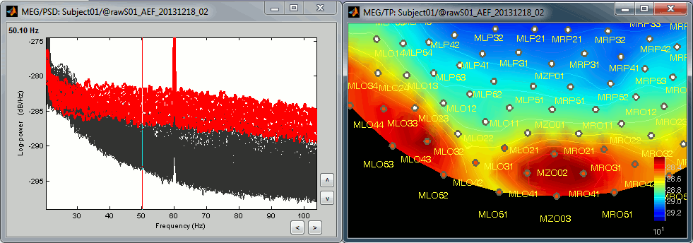
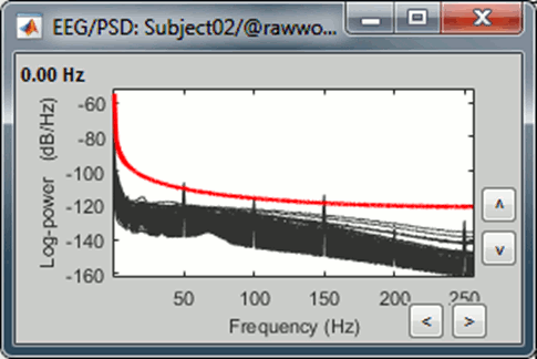
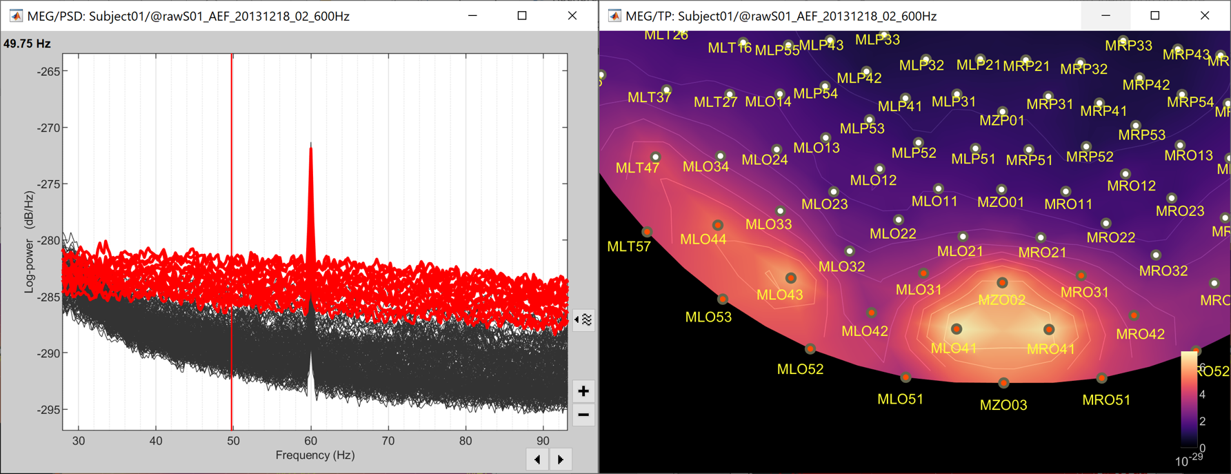
The power spectrum density (PSD) is usually a good way to spot a few bad channels, this is why we always recommend to compute it for all the datasets:

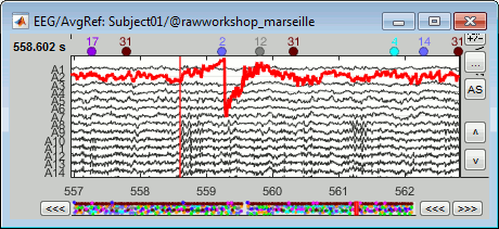
Simply looking at the signals traces, some channels may appear generally noisier than the others:
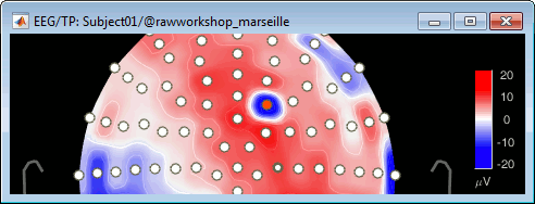
Looking at a 2D sensor topography, if one sensor shows very different values from its neighbors for extended periods of time, you can doubt of its quality:
Selecting sensors
- Double-click on the recordings for run #01 to open the MEG sensors.
Right-click on the time series figure > View topography (or press Ctrl+T).
Right-click on the topography figure > Channels > Display sensors (or press Ctrl+E).
If you can't see anything because the topography figure is too small, you can change the way the figures are automatically arranged. In the top-right corner of the Brainstorm figure, select the menu "Window layout options > Tiled".
You can select one channel by clicking on its signal or on the dot representing it in the topography figure. Note that the sensor selection is automatically reported to the other figure.
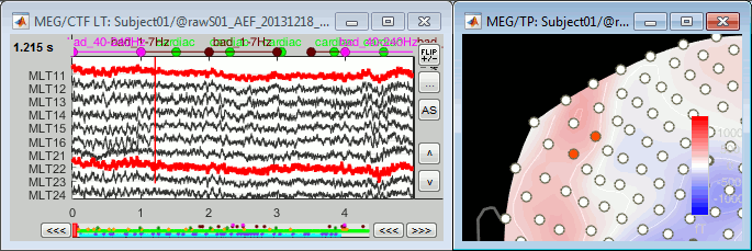
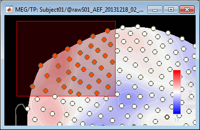
You can select multiple sensors at the same time the topography figure.
Right-click on the figure, then hold the mouse button and move the mouse.
Select a few sensors, then right-click on one of the figures and check out the Channels menu:
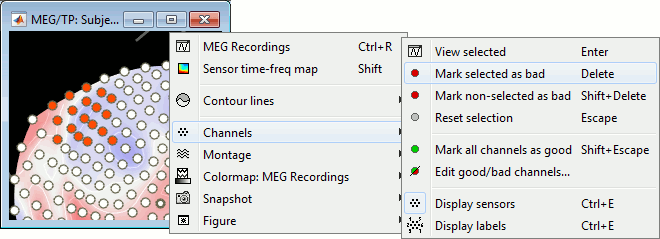
View selected: Show the time series of the selected sensors.
Mark selected as bad: Remove sensors from the display and all the further computations.
Mark non-selected as bad: Keep only the selected channels.
Reset selection: Unselect all the selected sensors.
Mark all channels as good: Brings back all the channels to display.
Edit good/bad channels: Opens an interface that looks like the channel editor, but with one extra column to edit the status (good or bad) of each channel.
Marking bad channels
Select a few channels, right-click > Channels > Mark selected as bad (or press the Delete key).
The selected channels disappear from the two views. In the time series figure, the signals are not visible anymore, in the topography the corresponding dots disappear and the values of the magnetic fields around the missing sensors get re-interpolated based on what is left.
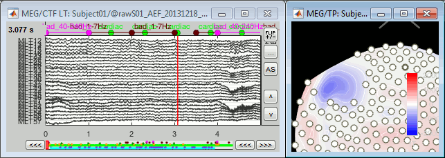
With the time series figure, you can display the signals that have been tagged as bad.
In the Record tab, select the montage "Bad channels".
In this view, you cannot select the channels, they are not available anymore.

Right-click on a figure > Channels > Edit good/bad channels.
This menu open a window very similar to the Channel Editor window, with additional green and red dots to indicate the status of each channel. Click on the dot to switch it to good or bad.

From the database explorer
Many options to change the list of bad channels are available from the database explorer.
The menus are available if you right-click one data file (or link to raw file). In this case, the selected operation is applied only on the selected file.

The same menus are also available for all the folders. In this case, the selected operation is applied recursively to all the data files (and links to raw files) that are found in the folder.

With this batching ability of the database explorer, you can quickly tag some bad channels in all the recordings of a subject or for the entire protocol. You can also get a quick overview of all the bad channels in all the files at once with the menu View all bad channels.

Restore all the good channels before moving to the next tutorial. For instance, right-click on the protocol folder TutorialIntroduction > Good/bad channels > Mark all channels as good.
Epoching and averaging
The list of bad channels is saved separately for each dataset.
At this stage of the analysis, the database contains only links to continuous files. When you import epochs from a continuous file, the list of bad channels will be copied from the raw file to all the imported data files.
Then you will be able to redefine this list for each epoch individually, tagging more channels as bad, or including back the ones that are ok. This way it is possible to exclude from the analysis the channels that are too noisy in a few trials only, for instance because of some movement artifacts.
When averaging, if an epoch contains one bad channel, this bad channel is excluded from the average but all the other channels are kept. If the same channel is good in other trials, it will be considered as good in the average. This means that not all the channels have the same number of trials for calculating the average.
This may cause the different channels of an averaged file to have different signal-to-noise ratios, which may lead to confusing results. However, we decided to implement the average in this way to be able to keep more data in the studies with a low number of trials and a lot of noise.
On the hard drive
The list of bad channels is saved for each data file separately, in the field ChannelFlag.
This vector indicates for each channel #i if it is good (ChannelFlag(i)= 1) or bad (ChannelFlag(i)= -1).
Right-click on a link to a continuous file > File > View file contents:
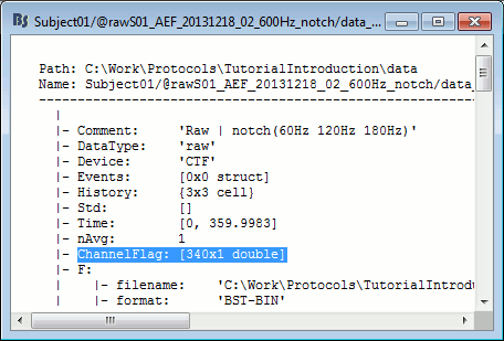
This information is duplicated in the sFile structure (F field) in order to be passed easily to the low-level reading functions. If you are planning to modify the list of bad channels manually, you need to change two fields: mat.ChannelFlag and mat.F.channelflag
