
|
Size: 21920
Comment:
|
Size: 21914
Comment:
|
| Deletions are marked like this. | Additions are marked like this. |
| Line 126: | Line 126: |
| * '''''right:MCB: F-statistics var(b)/var(Unconstr)|10.0_290.0ms''': This file saved the spatiotemporal dynamics of F-statistics between 10.0 and 290.0 ms. The abbreviations for ''F-statistics window size'',''temporal resolution'', and ''baseline'' is ''ws'', ''tr,'' and'' bs''. Click on this file. Choose ''Surface'' tab and set ''Data options > Amplitude'' to be '''50'''%. Right click on the pop-out window. Select S''napshot > Time contact sheet: Figure''.<<BR>><<BR>> {{attachment:MCBSnapshotSettting.png}} <<BR>><<BR>>''In this window, set ''Start time (ms)'' to be '''10''', ''End time (ms)'' to be '''290''', and ''Number of snapshots'' to be '''29'''. Click on ''Ok''.'' ''You will obtain the following figures. <<BR>><<BR>>''''' {{attachment:MCBFdynamicsRight.png||height="397",width="514"}} '''''<<BR>><<BR>>These figures display the F-statistics maps between 10 ms and 290 ms with 10-ms time interval. The baseline used in this example was set to be -104.2 ~ -10 ms. '' '' | * '''right:MCB: F-statistics var(b)/var(Unconstr)|10.0_290.0ms''': This file saved the spatiotemporal dynamics of F-statistics between 10.0 and 290.0 ms. The abbreviations for ''F-statistics window size,temporal resolution, ''and'' baseline'' is ''ws, tr, ''and'' bs''. Click on this file. Choose ''Surface'' tab and set ''Data options > Amplitude'' to be '''50'''%. Right click on the pop-out window. Select ''Snapshot > Time contact sheet: Figure''.''<<BR>><<BR>> {{attachment:MCBSnapshotSettting.png}} <<BR>><<BR>>''In this window, set ''Start time (ms)'' to be '''10''', ''End time (ms)'' to be '''290''', and ''Number of snapshots'' to be '''29'''. Click on ''Ok''.'' ''You will obtain the following figures. <<BR>><<BR>>''''' {{attachment:MCBFdynamicsRight.png||height="397",width="514"}} '''''<<BR>><<BR>>These figures display the F-statistics maps between 10 ms and 290 ms with 10-ms time interval. The baseline used in this example was set to be -104.2 ~ -10 ms. '' '' |
| Line 140: | Line 140: |
| 1. ''Chen YS, Cheng CY, Hsieh JC, Chen LF (2006)<<BR>>'''''[[http://www.ncbi.nlm.nih.gov/pubmed/16941832|Maximum contrast beamformer for electromagnetic mapping of brain activity]]'''''<<BR>>IEEE Transactions on Biomedical Engineering 53(9): 1765-1774.''''''' ''''''' ''' ''' '' ''' ''' ''' ''' | 1. ''Chen YS, Cheng CY, Hsieh JC, Chen LF (2006)<<BR>>'''''[[http://www.ncbi.nlm.nih.gov/pubmed/16941832|Maximum contrast beamformer for electromagnetic mapping of brain activity]]'''''<<BR>>IEEE Transactions on Biomedical Engineering 53(9): 1765-1774.' ' ''' ''' '' ''' ''' ''' ''' |
| Line 143: | Line 143: |
| ''<<EmbedContent(http://neuroimage.usc.edu/bst/get_feedback.php?Tutorials/Beamformers)>>''''' '' ''''''' ''' ''' '' ''' ''' | ''<<EmbedContent(http://neuroimage.usc.edu/bst/get_feedback.php?Tutorials/Beamformers)>>''''' '' ''''''''''' ''' ''' '''''''' ''' ''' ''' |
Beamforming methods
Authors: Hui-Ling Chan, Francois Tadel, Sylvain Baillet
The estimation of source distribution is an important step to understand the brain activity from EEG and MEG data. Dipole fitting, minimum norm estimation and beamformer are three commonly used methods. It has been proved that beamforming methods provide good spatial resolution. This tutorial will show how to apply beamforming methods to MEG data and obtain the statistic map of source activation.
We are going to use the protocol TutorialRaw created in the introduction tutorials. If you have not followed these tutorials yet, please do it now.
Contents
Introduction
Beamforming methods scan each targeted source position
latex error! exitcode was 2 (signal 0), transscript follows:and estimate the spatial filter
latex error! exitcode was 2 (signal 0), transscript follows:. By multiplying with the MEG recordings
latex error! exitcode was 2 (signal 0), transscript follows:, the spatial filter
latex error! exitcode was 2 (signal 0), transscript follows:outputs the temporal waveform
latex error! exitcode was 2 (signal 0), transscript follows:of the dipole source at that position with the dipole orientation
latex error! exitcode was 2 (signal 0), transscript follows:as below:
latex error! exitcode was 2 (signal 0), transscript follows:
where 'T' indicates the transpose of a matrix or vector. The beamforming spatial filter can be vector-type or scalar-type.
Vector-type beamformer
For each position
latex error! exitcode was 2 (signal 0), transscript follows:, three orthogonal spatial filters
latex error! exitcode was 2 (signal 0), transscript follows:are computed by applying the unit-gain constraint as well as the minimum norm and minimum variance criteria as below [Van Veen et al., 1997]:
latex error! exitcode was 2 (signal 0), transscript follows:
where
latex error! exitcode was 2 (signal 0), transscript follows:is the covariance matrix of MEG recordings during window
latex error! exitcode was 2 (signal 0), transscript follows:,
latex error! exitcode was 2 (signal 0), transscript follows:is the identity matrix,
latex error! exitcode was 2 (signal 0), transscript follows:is the gain matrix for the dipole located at position
latex error! exitcode was 2 (signal 0), transscript follows:, and
latex error! exitcode was 2 (signal 0), transscript follows:is the regularization parameter which compromises the minimum norm and minimum variance criteria.
Scalar-type beamformer
For each position
latex error! exitcode was 2 (signal 0), transscript follows:, the source orientation
latex error! exitcode was 2 (signal 0), transscript follows:is first estimated to enable the spatial filter to output the source activity with maximum power or fitting some other criteria. The dipole orientation can be obtained by exhaustive search, non-linear search [Robinson and Vrba, 1999], or analytical solution [Chen et al., 2006]. The estimated dipole orientation
latex error! exitcode was 2 (signal 0), transscript follows:is then applied to calculate the spatial filter as follows [Robinson and Vrba, 1999]:
latex error! exitcode was 2 (signal 0), transscript follows:
LCMV beamformer
LCMV stands for linearly-constrained minimum variance. LCMV beamformer is vector-type beamformer. For each position
latex error! exitcode was 2 (signal 0), transscript follows:, this method calculates the neural activity index, which is interpreted as the estimate of source to noise variance.
Neural activity index
For each position
latex error! exitcode was 2 (signal 0), transscript follows:, the variance of source activity during active state
latex error! exitcode was 2 (signal 0), transscript follows:is calculated as follows:
latex error! exitcode was 2 (signal 0), transscript follows:
or
latex error! exitcode was 2 (signal 0), transscript follows:
where
latex error! exitcode was 2 (signal 0), transscript follows:is the covariance matrix computed from MEG recordings during active state
latex error! exitcode was 2 (signal 0), transscript follows:and
latex error! exitcode was 2 (signal 0), transscript follows:indicates the maximum eigenvalue of the expression in braces.
When the location
latex error! exitcode was 2 (signal 0), transscript follows:is far from sensors, the elements of lead field matrix
latex error! exitcode was 2 (signal 0), transscript follows:are small. So the elements of
latex error! exitcode was 2 (signal 0), transscript follows:are generally large and the estimated variance for the deep source becomes large. When the location
latex error! exitcode was 2 (signal 0), transscript follows:is close to sensors, the elements of lead field matrix
latex error! exitcode was 2 (signal 0), transscript follows:are large. It results in small values of the elements of
latex error! exitcode was 2 (signal 0), transscript follows:and small estimated variance for the superficial source. To reduce the effect caused by the depth of source location, the estimated source variance
latex error! exitcode was 2 (signal 0), transscript follows:is normalized by the noise variance
latex error! exitcode was 2 (signal 0), transscript follows:as follows:
latex error! exitcode was 2 (signal 0), transscript follows:
or
latex error! exitcode was 2 (signal 0), transscript follows:
where
latex error! exitcode was 2 (signal 0), transscript follows:is the covariance matrix computed from MEG recordings during control state
latex error! exitcode was 2 (signal 0), transscript follows:. The normalized variance
latex error! exitcode was 2 (signal 0), transscript follows:is called neural activity index (NAI).
LCMV process
Drag and drop all of the epochs in Subject01 / right / right | timeoffset (98 files) into Process1.
Click on [RUN] and select the process "Sources > LCMV Beamformer".
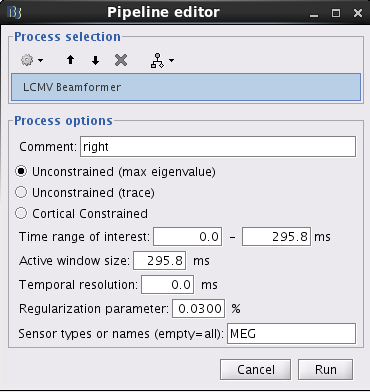
With this window you can select the method you want to use to estimate the source variance and noise variance, the time window of active state, the regularization parameter, and the sensors you are going to use for this estimation. You can edit the following options:
Comment: This field contains what is going to be displayed in the database explorer.
Method: Please select Unconstrained (max eigenvalue) or Unconstrained (trace). The method Unconstrained (max eigenvalue) calculates the variances of source activity and noise by using the maximum eigenvalue. The method Unconstrained (trace) calculates the variances of source activity and noise by using trace. The method Cortial Constrained use the orientation of cortical surface as dipole orientation. Note that the method Cortial Constrained is only available when the Head Model provides the orientation for each grid location. The unconstrained methods may give more smooth results than the cortical constrained method.
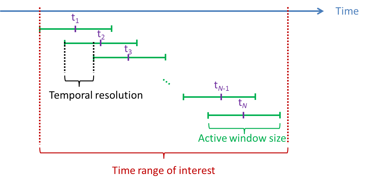
Time window of active state: Three parameters have to be set: Time range of interest, Active window size, and Temporal resolution. The neural activity index is computed using the variance of source activity during active state
latex error! exitcode was 2 (signal 0), transscript follows:
. Active window size defines the duration of active state. Large active window size (at least larger than the number of sensors) is recommended. The time window of active state is going to be slided in Time range of interest with the interval set to be Temporal resolution. If there are multiple active state windows, the time label of the neural activity index will be set as the middle time of each active state window, that is,latex error! exitcode was 2 (signal 0), transscript follows:
in the following figure. You are going to obtain the spatiotemporal F-statistics bewteenlatex error! exitcode was 2 (signal 0), transscript follows:
andlatex error! exitcode was 2 (signal 0), transscript follows:
.
Regularization parameter: This value will be multiplied with the maximum eigenvalue of the covariance matrix computed from the recordings during Time range of interest. The larger value of regularization parameter may give the more smooth results.
Sensors type: Modalities that are used for the reconstruction. Here we only have one type of MEG sensors, so nothing to change.
Click on Run.
Two new files are available in the database explorer.
right: LCMV: spatial filter(Unconstr)|0.0_295.8ms: This file saves the three orthogonal spatial filters for each dipole position. These spatial filters are normalized by the standard deviation of noise. Note that there is one spatial filter for each dipole location if the method Cortically Constrained is used.
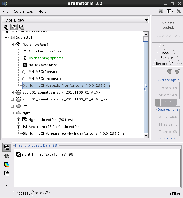
right: LCMV: neural activity index(Unconstr)|0.0_295.8ms: This file saves the neural activity index for every dipole position.
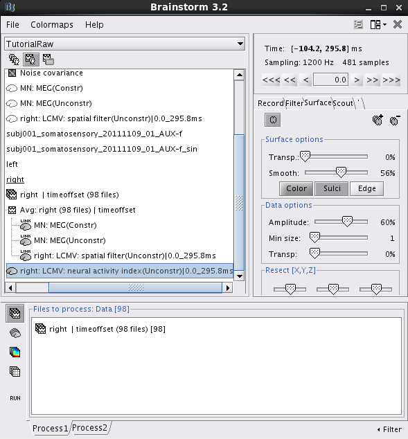
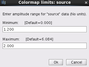
Double click on this file. Right click on anywhere of the pop-out window. From the pop-out menu, select Colormap:Sources > Maximum: Custom.... Set Minimum to be 1.2 and Maximum to be 2.0. Click Ok.
Set the time to be anytime between 0 and 295.8 ms. Then click Surface tab on the right panel of database explorer. Set Data options > Amplitude to be 50%.
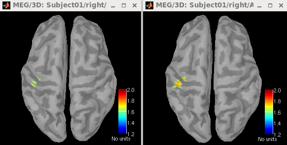
The maps of neural activity index estimated using Unconstrained (trace) and Unconstrained (max eigenvalue) are shown in the left and right figures, respectively. Both maps display strong activations in the left sensory area.
Maximum constrast beamformer
Maximum constrast beamformer (MCB) is scalar-type beamformer. For each position
latex error! exitcode was 2 (signal 0), transscript follows:, it provides an analytical solution of dipole orientation
latex error! exitcode was 2 (signal 0), transscript follows:, which maximizes the constrast of beamformer outputs between active state and control state as bellow:
latex error! exitcode was 2 (signal 0), transscript follows:
where
latex error! exitcode was 2 (signal 0), transscript follows:is the covariance matrix computed from the measurements during active state and
latex error! exitcode was 2 (signal 0), transscript follows:is the covariance matrix computed from the measurements during control state.
Solution of dipole orientation
The solution of spatial filter can be rewritten as
latex error! exitcode was 2 (signal 0), transscript follows:
where both
latex error! exitcode was 2 (signal 0), transscript follows:and
latex error! exitcode was 2 (signal 0), transscript follows:depend only on the dipole location
latex error! exitcode was 2 (signal 0), transscript follows:. Then the objective function for obtaining the dipole orientation
latex error! exitcode was 2 (signal 0), transscript follows:can be rewritten as
latex error! exitcode was 2 (signal 0), transscript follows:
where both of the 3-by-3 matrices
latex error! exitcode was 2 (signal 0), transscript follows:and
latex error! exitcode was 2 (signal 0), transscript follows:does not depend on the dipole orientation
latex error! exitcode was 2 (signal 0), transscript follows:. The solution of dipole orientation
latex error! exitcode was 2 (signal 0), transscript follows:is the eigenvector corresponding to the maximum eigenvalue of the matrix
latex error! exitcode was 2 (signal 0), transscript follows:.
Statistical mapping
After obtaining the dipole orientation
latex error! exitcode was 2 (signal 0), transscript follows:and the spatial filter
latex error! exitcode was 2 (signal 0), transscript follows:for dipole position
latex error! exitcode was 2 (signal 0), transscript follows:, the F-statistic value at time
latex error! exitcode was 2 (signal 0), transscript follows:can be obtained using the following formula:
latex error! exitcode was 2 (signal 0), transscript follows:
where
latex error! exitcode was 2 (signal 0), transscript follows:is the covariance matrix computed from the measurements during window
latex error! exitcode was 2 (signal 0), transscript follows:,
latex error! exitcode was 2 (signal 0), transscript follows:is the size of
latex error! exitcode was 2 (signal 0), transscript follows:, and the range of
latex error! exitcode was 2 (signal 0), transscript follows:is
latex error! exitcode was 2 (signal 0), transscript follows:.
latex error! exitcode was 2 (signal 0), transscript follows:is a segment of active state
latex error! exitcode was 2 (signal 0), transscript follows:. The meaning of F-statistic is the same as the normalized variance
latex error! exitcode was 2 (signal 0), transscript follows:used in LCMV beamforming method.
If the number of
latex error! exitcode was 2 (signal 0), transscript follows:is small, the peak of temporal dynamics of F-statistic value may shift. In this case, it is more appropriate to replace the covariance matrix
latex error! exitcode was 2 (signal 0), transscript follows:with
latex error! exitcode was 2 (signal 0), transscript follows:
or
latex error! exitcode was 2 (signal 0), transscript follows:
where
latex error! exitcode was 2 (signal 0), transscript follows:represents the window of baseline and its size is
latex error! exitcode was 2 (signal 0), transscript follows:. When
latex error! exitcode was 2 (signal 0), transscript follows:is used, the F-statistic value represents the estimate of source power to noise variance.
MCB process
Drag and drop all of the epochs in Subject01 / right / right | timeoffset (98 files) into Process1.
Click on [RUN] and select the process "Sources > Maximum Contrast Beamformer".
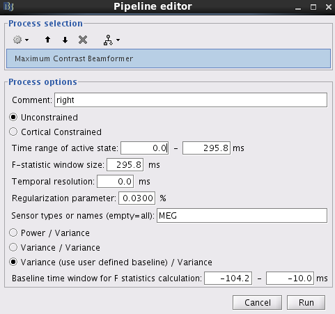
With this window you can select the dipole orientation you want to use, the time window of active state, the window size you are going to use for F-statistics computation, the regularization parameter, and the sensors you are going to use for this estimation. You can edit the following options:
Comment: This field contains what is going to be displayed in the database explorer.
Dipole orientation: Please select Unconstrained, which calculates the dipole orientation using the maximum contrast criterion. The method Cortial Constrained uses the orientation of cortical surface as dipole orientation. Note that the method Cortial Constrained is only available when the Head Model provides the orientation for each grid location. The unconstrained method may give more smooth results than the cortical constrained method.
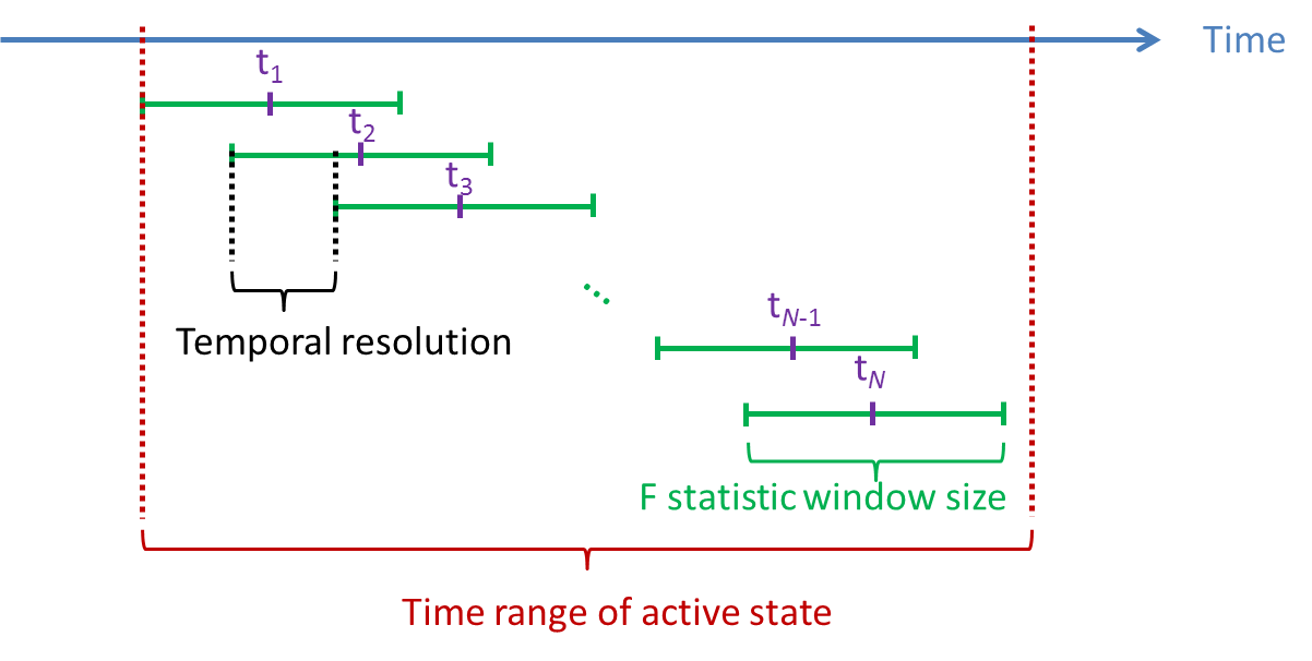
Time windows: Three parameters have to be set: Time range of active window, F statistic window size, and Temporal resolution. The dipole orientation and spatial filter is estimated using the variance of source activity during active state
latex error! exitcode was 2 (signal 0), transscript follows:
. F statistic window size defines the length of the window for F-statistic computation, that is,latex error! exitcode was 2 (signal 0), transscript follows:
. The time window for computing F statistics is going to be slided in Time range of active state with the interval set to be Temporal resolution. If there are more than one F statistic windows, the time label of the F statistics will be set as the middle time of each window, that is,latex error! exitcode was 2 (signal 0), transscript follows:
in the following figure. And you will obtain the spatiotemporal F-statistics bewteenlatex error! exitcode was 2 (signal 0), transscript follows:
andlatex error! exitcode was 2 (signal 0), transscript follows:
.
Regularization parameter: This value will be multiplied with the maximum eigenvalue of the covariance matrix computed from the recordings during Time range of interest. The larger value of regularization parameter may give the more smooth results.
Sensors type: Modalities that are used for the reconstruction. Here we only have one type of MEG sensors, so nothing to change.
Method for F statistic computation: Please select Variance (use user define baseline) / Variance to compute F statistic values. The other two methods are Power / Variance and Variance (use user defined baseline) / Variance. When the methiod Variance (use user defined baseline) / Variance is selected, the field of Baseline time window for F ststistics calculation must be given. In this example, we set the baseline to be -104.2 to -10 ms.
Click on Run.
Two new files are available in the database explorer.
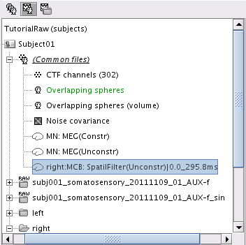
right:MCB: SpatilFilter(Unconstr)|0.0_295.8ms: This file saved the spatial filter for each grid point. The spatial filters are normalized using the standard deviation of beamformer outpouts during control state.
right:MCB: F-statistics var(b)/var(Unconstr)|0.0_295.8ms: This file saved the F-statistic value for each grid point during 0-295.8 ms.
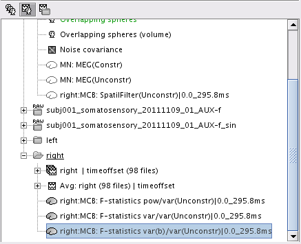
Double click on this file. Set the time to be anytime between 0 and 295.8 ms. Then click Surface tab on the right panel of database explorer. Set Data options > Amplitude to be 95%.
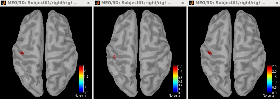
From left to right, the figures display the F statistics computed using Power / Variance, Variance / Variance, and Variance (use user defined baseline) / Variance. The baseline used in this example was set to be -104.2 ~ -10 ms.
Process Subject01 / left / left | timeoffset (101 files) using the same procedure.
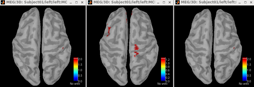
From left to right, the figures display the F statistics computed using Power / Variance, Variance / Variance, and Variance (use user defined baseline) / Variance. The baseline used in this example was set to be -104.2 ~ -10 ms.
Process Subject01 / right / right | timeoffset (98 files) using the following parameter values to obtain the spatiotemporal dynamics of F-statistics.
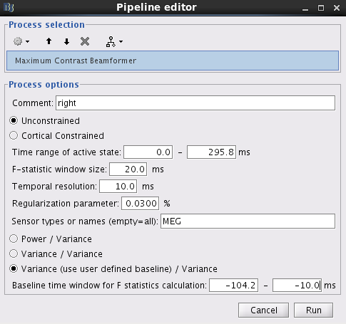
Two new files are available in Database explorer:right:MCB: SpatilFilter(Unconstr)|0.0_295.8ms: This file saves the spatial filter for each grid points. The filename shows the time range used to compute spatial filters, that is, 0.0 to 295.8 ms in this case.
right:MCB: F-statistics var(b)/var(Unconstr)|10.0_290.0ms: This file saved the spatiotemporal dynamics of F-statistics between 10.0 and 290.0 ms. The abbreviations for F-statistics window size,temporal resolution, and baseline is ws, tr, and bs. Click on this file. Choose Surface tab and set Data options > Amplitude to be 50%. Right click on the pop-out window. Select Snapshot > Time contact sheet: Figure.
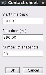
In this window, set Start time (ms) to be 10, End time (ms) to be 290, and Number of snapshots to be 29. Click on Ok. You will obtain the following figures.
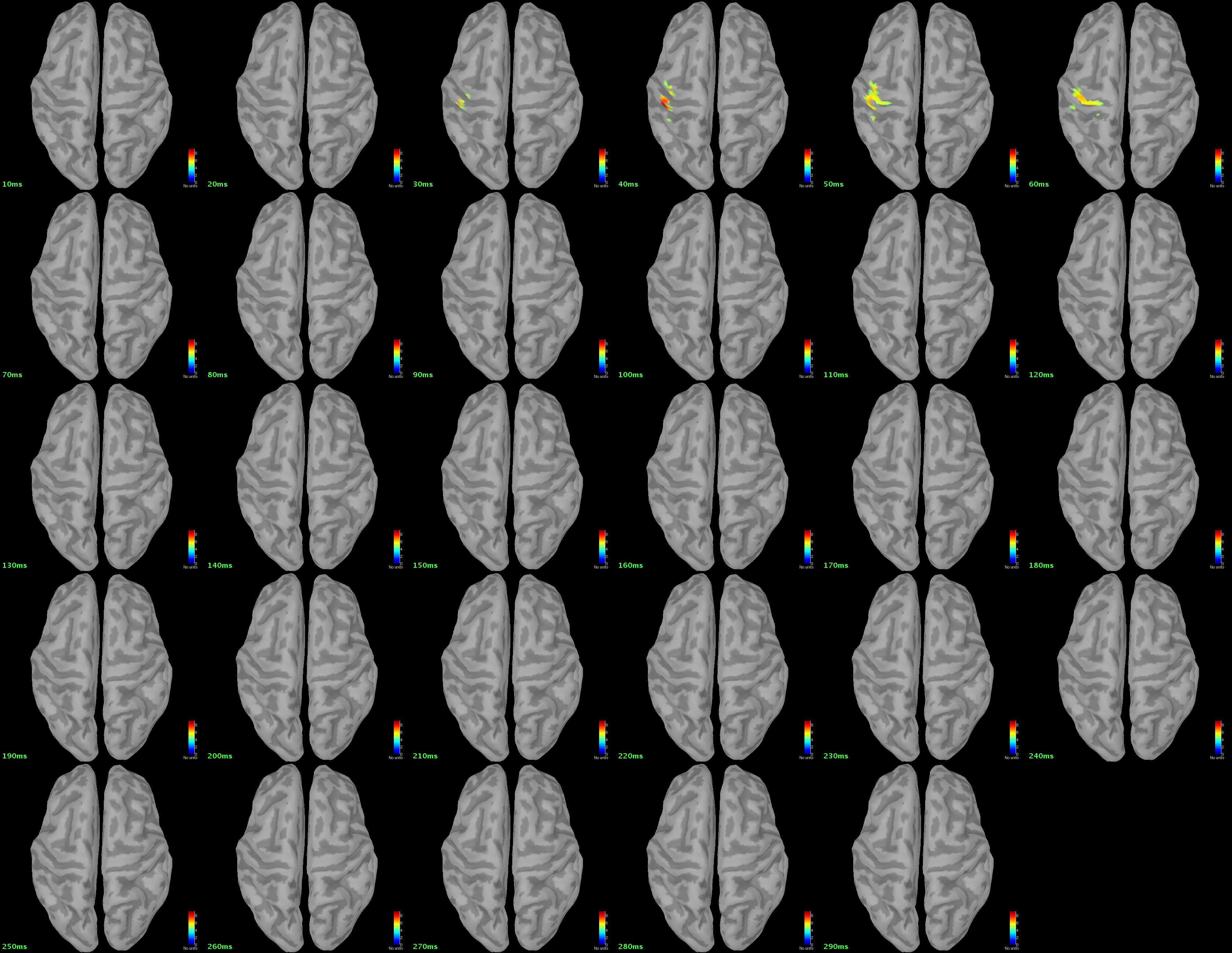
These figures display the F-statistics maps between 10 ms and 290 ms with 10-ms time interval. The baseline used in this example was set to be -104.2 ~ -10 ms.
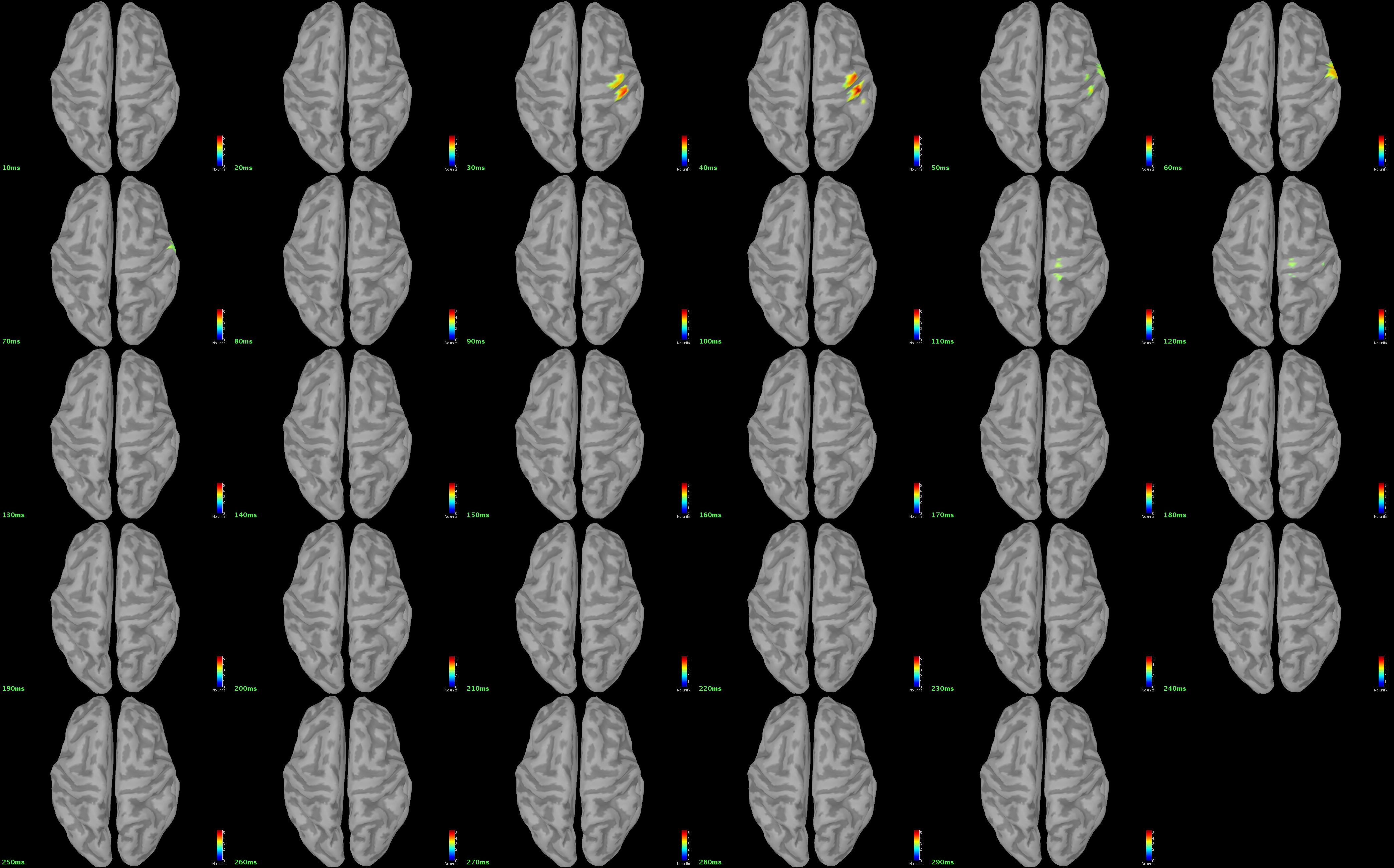
Process Subject01 / left / left | timeoffset (98 files) with the same parameter values used in the previous step to obtain the spatiotemporal dynamics of F-statistics.
Beamformer-based correlation/coherence imaging
Dynamic imaging of coherent sources (DICS)
[Under construction]
Spatiotemporal imaging of linearly-related source components (SILSC)
[Under construction]
References
Van Veen BD, Van Drongelen W, Yuchtman M, Suzuki A (1997)
Localization of brain electrical activity via linearly constrained minimum variance spatial filtering
IEEE Transactions on Biomedical Engineering 44(9): 867-880.Robinson SE and Vrba J (1999)
Functional neuroimaging by synthetic aperture magnetometry
Recent Advances in Biomagnetism. Tohoku University Press 1999: 302-305.Chen YS, Cheng CY, Hsieh JC, Chen LF (2006)
Maximum contrast beamformer for electromagnetic mapping of brain activity
IEEE Transactions on Biomedical Engineering 53(9): 1765-1774.' '
Feedback