|
Size: 5779
Comment:
|
Size: 5770
Comment:
|
| Deletions are marked like this. | Additions are marked like this. |
| Line 15: | Line 15: |
| 1. Do the same for the low-resolution cortex surface (Subject01/cortex_300000V). This is the downsampled version of the same thing. You can click on the "Edge" button on the surface tab to see the same triangulation as you would see when displaying the low-resolution cortex surface.<<BR>><<BR>>{{attachment:sphereSubj.gif}} | 1. Do the same for the low-resolution cortex surface (Subject01/cortex_300000V). This is the downsampled version of the same thing. You can click on the "Edge" button on the surface tab to see the same triangulation as you would see when displaying the low-resolution cortex surface.<<BR>><<BR>> {{attachment:sphereSubj.gif}} |
| Line 20: | Line 20: |
| == Those menus don't show up == | == It doesn't work == |
Group studies: Subject co-registration
In the typical Brainstorm workflow, you process each subject individually: you have access to the MRI of the subject, you extract the cortex envelope from it using the software of your choice (FreeSurfer, BrainVISA, BrainSuite or CIVET), you import the recordings and estimate the sources for each subject separately.
After importing and pre-processing all the individual information, you will probably be interested in calculating some group statistics, to extract the significant features across all the subjects in your study. in order to do this at the source level, all the source files must be using the same support cortex source (= the same source space). The problem you typically face is that the shape and number of vertices of the cortex surface varies across subject: one source index doesn't mean the same thing for all the subjects, hence it's impossible to compare them directly.
The solution is to reproject the sources of all the subjects on the default anatomy. The reprojected versions share the same source space, the cortex from Colin27 anatomy, so they can be averaged or used to calculate any other statistics across subjects. Different methods are available in Brainstorm depending on the software you are using for the MRI segmentation. The recommended option is to use FreeSurfer and benefit from the very efficient registration system this software offers.
Using FreeSurfer registered spheres
The FreeSurfer software registers all the subjects to the FSAverage atlas using a spherical representation of each hemisphere. The hemisphere of the subject's brain are inflated to a sphere, then this sphere is deformed to match the curvature map of the equivalent sphere in the FSAverage subject. The result of this registration is saved in the FreeSurfer output folder in surf/lh.sphere.reg and surf/rh.sphere.reg.
We can illustrate this method using the protocol TutorialRaw, that you created while reading the introduction tutorials.
Select the protocol TutorialRaw, go the anatomy view
Right-click on the high-resolution cortex surface (Subject01/cortex_300000V) > MRI registration > View FreeSurfer sphere. Those two spheres represent the inflated left and the right hemispheres, registered on the FSAverage subject. The darker stripes represent the bottom of the sulci: the map is exactly the same as the one that is displayed on the cortex surface when you click on the "Sulci" button in the Surface tab.
Do the same for the low-resolution cortex surface (Subject01/cortex_300000V). This is the downsampled version of the same thing. You can click on the "Edge" button on the surface tab to see the same triangulation as you would see when displaying the low-resolution cortex surface.

- Now do the same for the high-resolution cortex of the default anatomy.
The best available option is selected automatically
It doesn't work
If you have started your analysis before those options were made available in Brainstorm
A cheap alternative
If you did not process your MRI files with FreeSurfer, or if you are working with an older database, you have another option available to re-project your subject's source maps on the default anatomy. The results are much less reliable, but the method is quite robust and can be used for all sorts of purposes. We can illustrate this method using the protocol TutorialCTF, that you created while reading the introduction tutorials.
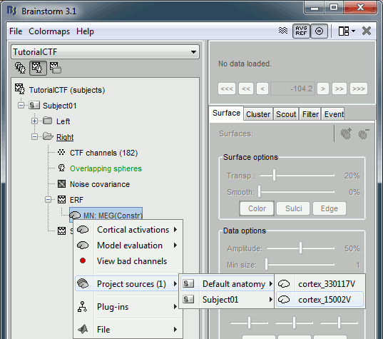
Right-click on Subject01/Right/MN > Project sources > Default anatomy > Cortex_15000V
- The source cortex (Subject01) and the destination cortex (Colin27) are split in two hemispheres, and then for each hemisphere:
- Alignment along the anterior commissure/posterior commissure axis
- Smooth intensly to keep only the main featuresof the surfaces
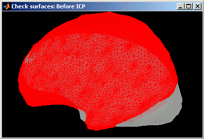
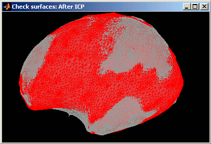
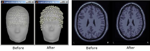
Deformation of the individual surface to match the Colin27 surface with an iterative closest point algorithm (ICP). The following figures show the left hemispheres before and after the ICP deformation:
- Interpolation of the source amplitudes from the subject surface to the Colin27 surface using Shepard’s method (weighted combination of a few nearest neighbors)
The interpolation matrix subject->Colin is computed only once and then saved in the subject's cortex surface file, in the field "tess2tess_interp"
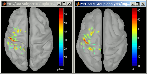
You can see that a new subject and a new condition were created in the database, that contain the sources from Subject01/Right/ERF projected on the default anatomy:
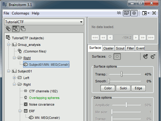
Display at the same time the original source file and the projected one to see how it looks like (left: Subject01, right: Colin)
- Delete the "Group analysis" subject.
Warped brains
It is important to note that pseudo-individual anatomies that were generated by deforming the Colin27 brain using the digitized head points do not need to be re-projected on the default anatomy.
If you have two subjects for which you generated pseudo anatomies using the popup menu Digitized head points > Warp > Deform default anatomy to fit these points, you can directly use their source maps for computing any statistics or difference. You don't need to use this menu "Project sources".
Feedback
