|
Size: 7298
Comment:
|
Size: 7364
Comment:
|
| Deletions are marked like this. | Additions are marked like this. |
| Line 4: | Line 4: |
| This tutorial illustrates how to use the functions developed at Aude Oliva's lab (MIT) to run support vector machine (SVM) and linear discriminant analysis (LDA) classification on your MEG data across time. | This tutorial illustrates how to use the functions developed at Aude Oliva's lab (MIT, CSAIL), and McGovern's MEG lab (Dimitrios Pantazis's lab) to run support vector machine (SVM) and linear discriminant analysis (LDA) classification on your MEG data across time. |
| Line 16: | Line 16: |
| These two processes work in very similar ways: | These two processes work in a similar way: |
| Line 20: | Line 20: |
| * Two methods are offered for the classification of MEG recordings across time: Support vector machine (SVM) and Linear discriminant analysis (LDA). | * '''Classifier''': Two methods are offered for the classification of MEG recordings across time: Support vector machine (SVM) and Linear discriminant analysis (LDA). |
| Line 58: | Line 58: |
| * '''Matlab SVM/LDA''': Require Matlab's Statistics and Machine Learning Toolbox. <<BR>><<BR>>These methods do a k-fold stratified cross-validation for you, meaning that each fold will contain the same proportions of the two types of class labels (option "Number of folds"). | * '''Matlab SVM/LDA''': Require Matlab's Statistics and Machine Learning Toolbox. <<BR>>These methods do a k-fold stratified cross-validation for you, meaning that each fold will contain the same proportions of the two types of class labels (option "Number of folds"). |
Decoding conditions
Authors: Seyed-Mahdi Khaligh-Razavi, Francois Tadel, Dimitrios Pantazis
This tutorial illustrates how to use the functions developed at Aude Oliva's lab (MIT, CSAIL), and McGovern's MEG lab (Dimitrios Pantazis's lab) to run support vector machine (SVM) and linear discriminant analysis (LDA) classification on your MEG data across time.
Contents
License
The decoding tutorial dataset remains a property of Aude Oliva’s Lab, Computer Science and AI (CSAIL), Massachusetts Institute of Technology, Cambridge, US. Its use and transfer outside the Brainstorm tutorial, e.g. for research purposes, is prohibited without written consent from the Lab.
If you reference this dataset in your publications, please acknowledge its authors (Seyed-Mahdi Khaligh-Razavi and Dimitrios Pantazis) and cite Khaligh-Razavi et al. (2015). For questions, please contact us through the Brainstorm forum.
Presentation of the experiment
- One subject, one acquisition run of 15 minutes.
- The subject performs an orthogonal image categorization task.
- During this run, the participant saw:
- 720 stimuli (360 faces, 360 scenes)
- Images centrally-presented (6 degree visual angle)
- Presentation duration of each image: 500ms
- The subject has to decide for each image (without responding) if:
- scenes were indoor / outdoor
- faces were male / female
Response: Every 2 to 4 trials (randomly determined), a question mark would appear on the screen for 1 second. At this time, participants were asked to press a button to indicate the category of the last image (male/female, indoor/outdoor), and they were also allowed to blink/swallow. This task was designed to ensure participants were attentive to the images without explicitly encoding them into memory. Participants only responded during the “question mark” trials so that activity during stimulus perception was not contaminated by motor activity.
Fixation: During the task, participants were asked to fixate on a cross centered on the screen and their eye movements were tracked, to ensure any results were not due to differential eye movement patterns.
Context: The whole experiment was divided into 16 runs. Each run contained 45 randomly selected images (each of them shown twice per run—not in succession), resulting in a total experiment time of about 50 min. The MEG data that is included here for demonstration purposes contains only the first 15 minutes of the whole session, during which 53 faces and 54 scenes have been observed.
Ethics: The study was conducted according to the Declaration of Helsinki and approved by the local ethics committee (Institutional Review Board of the Massachusetts Institute of Technology). Informed consent was obtained from all participants.
MEG acquisition at 1000Hz with an Elekta-Neuromag Triux system
Description of the decoding functions
Two decoding processes are available in Brainstorm:
Decoding > Classification with cross-validation (process_decoding_crossval.m)
Decoding > Classification with permutation (process_decoding_permutation.m)
These two processes work in a similar way:
Input: the input is the channel data from two conditions (e.g. condA and condB) across time. Number of samples per condition should be the same for both condA and condB. Each of them should at least contain two samples.
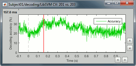
Output: the output is a decoding curve across time, showing your decoding accuracy (decoding condA vs. condB) at time point 't'.
Classifier: Two methods are offered for the classification of MEG recordings across time: Support vector machine (SVM) and Linear discriminant analysis (LDA).
In the context of this tutorial, we have two condition types: faces, and scenes. We want to decode faces vs. scenes using 306 MEG channels. In the data, the faces are named as condition ‘201’; and the scenes are named as condition ‘203’.
Download and installation
Go to the Download page of this website, and download the file: sample_decoding.zip
- Unzip it in a folder that is not in any of the Brainstorm folders (program folder or database folder). This is really important that you always keep your original data files in a separate folder: the program folder can be deleted when updating the software, and the contents of the database folder is supposed to be manipulated only by the program itself.
- Start Brainstorm (Matlab scripts or stand-alone version).
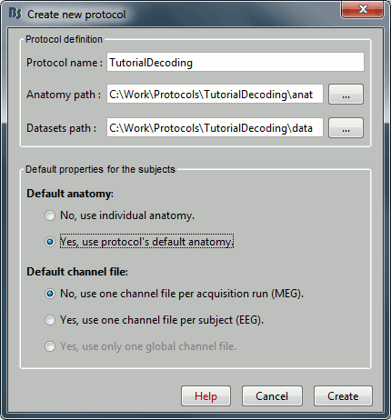
Select the menu File > Create new protocol. Name it "TutorialDecoding" and select the options:
"Yes, use protocol's default anatomy",
"No, use one channel file per condition".
Import the recordings
- Go to the "functional data" view (sorted by subjects).
Right-click on the TutorialDecoding folder > New subject > Subject01
Leave the default options you defined for the protocol.Right click on the subject node (Subject01) > Review raw file.
Select the file format: "MEG/EEG: Neuromag FIFF (*.fif)"
Select the file: sample_decoding/mem6-0_tsss_mc.fif

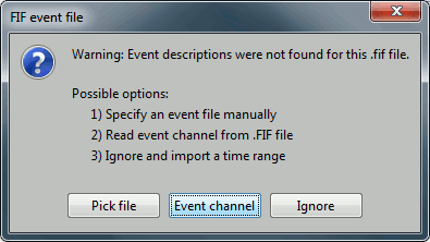
Select "Event channels" to read the triggers from the stimulus channel.
- We will not pay much attention to MEG/MRI registration because we are not going to compute any source models, the decoding is done on the sensor data.
Right-click on the "Link to raw file" > Import in database.
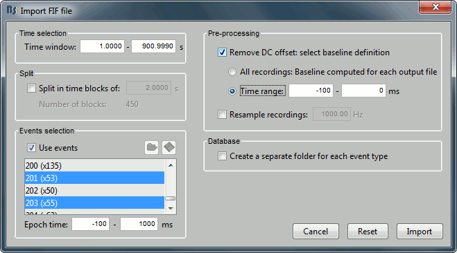
- Select only two events: 201 (faces) and 203(scenes)
- Epoch time: [-100, 1000] ms
- Remove DC offset: Time range: [-100, 0] ms
- Do not create separate folders for each event type
You will get a message saying "some epochs are shorter than the others". Answer yes.
Select files
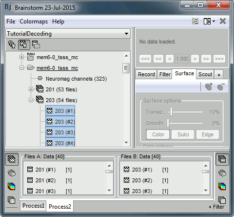
Select the Process2 tab at the bottom of the Brainstorm window.
Drag and drop 40 files from group 201 to the left (Files A).
Drag and drop 40 files from group 203 to the right (Files B).
You can select more than 40 or less. The important thing is that both ‘A’ and ‘B’ should have the same number of files.
Cross-validation
Cross-validation is a model validation technique for assessing how the results of our decoding analysis will generalize to an independent data set.
Select process "Decoding > Classification with cross-validation":
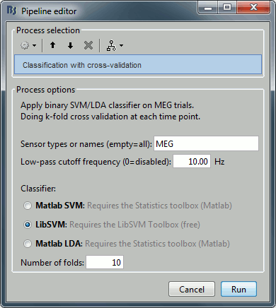
Low-pass cutoff frequency: If set, it will apply a low-pass filter to all the input recordings.
Matlab SVM/LDA: Require Matlab's Statistics and Machine Learning Toolbox.
These methods do a k-fold stratified cross-validation for you, meaning that each fold will contain the same proportions of the two types of class labels (option "Number of folds").LibSVM: Requires the LibSVM toolbox (download and add to your path).
The LibSVM cross-validation may be faster but will not be stratified.
The process will take some time. The results are then saved in a file in the new decoding folder.
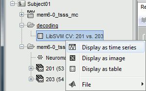
If you double click on it you will see a decoding curve across time.
Permutation
This is an iterative procedure. The training and test data for the SVM/LDA classifier are selected in each iteration by randomly permuting the samples and grouping them into bins of size n (you can select the trial bin sizes). In each iteration two samples (one from each condition) are left out for test. The rest of the data are used to train the classifier with.
Select process "Decoding > Classification with cross-validation". Set options as below:
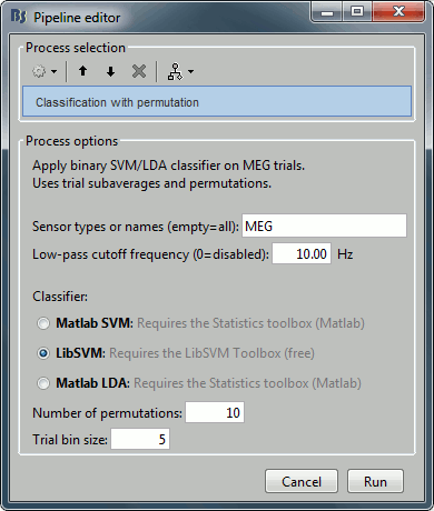
Trial bin size: If greater than 1, the training data will be randomly grouped into bins of the size you determine here. The samples within each bin are then averaged (we refer to this as sub-averaging); the classifier is then trained using the averaged samples. For example, if you have 40 faces and 40 scenes, and you set the trial bin size to 5; then for each condition you will have 8 bins each containing 5 samples. Seven bins from each condition will be used for training, and the two left-out bins (one face bin, one scene bin) will be used for testing the classifier performance.
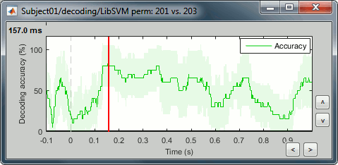
The results are saved in a file in the new decoding folder.
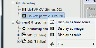
Right-click > Display as time series (or double click).
References
Khaligh-Razavi SM, Bainbridge W, Pantazis D, Oliva A (2015)
Introducing Brain Memorability: an MEG study (in preparation).Cichy RM, Pantazis D, Oliva A (2014)
Resolving human object recognition in space and time, Nature Neuroscience, 17:455–462.
