|
Size: 7271
Comment:
|
Size: 9368
Comment:
|
| Deletions are marked like this. | Additions are marked like this. |
| Line 14: | Line 14: |
| * Decoding > Classification with SVD * Decoding > Classification with max-correlation classifier |
* Decoding > SVM classifier decoding * Decoding > max-correlation classifier decoding |
| Line 31: | Line 31: |
| * "'''No, use one channel file per condition'''". <<BR>><<BR>> {{attachment:1_create_new_protocol.jpg||width="370"}} | * "'''No, use one channel file per condition'''". <<BR>><<BR>> {{attachment:1_create_new_protocol.jpg||width="400"}} |
| Line 36: | Line 36: |
| * Right click on the subject node (Subject01) > '''Review raw file'''''.'' <<BR>>Select the file format: "'''MEG/EEG: Neuromag FIFF (*.fif)'''"<<BR>>Select the file: sample_decoding/'''mem6-0_tsss_mc.fif''' <<BR>> {{attachment:2_review_raw_file.jpg||width="370"}} <<BR>>{{attachment:2_review_raw_file2.jpg||width="370"}} |
* Right click on the subject node (Subject01) > '''Review raw file'''''.'' <<BR>>Select the file format: "'''MEG/EEG: Neuromag FIFF (*.fif)'''"<<BR>>Select the file: '''subj04NN-sess01-0_tsss.fif''' <<BR>> * {{attachment:2_review_raw_file.jpg||width="440"}} <<BR>><<BR>> {{attachment:2_review_raw_file2.jpg||width="440"}} <<BR>><<BR>> * Select "Event channels" to read the triggers from the stimulus channel. <<BR>><<BR>> {{attachment:3_event_channel.jpg||width="320"}} * We will not pay attention to MEG/MRI registration because we are not going to compute any source models. The decoding is done on the sensor data. * Double click on the 'Link to raw file' to visualize the raw recordings. Event codes 13-24 indicate responses to face images, and we will combine them to a single group called 'faces'. To do so, select events 13-24 and from the menu select "'''Events > Duplicate groups'''". Then select "'''Events > Merge groups'''". The event codes are duplicated first so we do not lose the original 13-24 event codes. {{attachment:4_duplicate_groups_faces.jpg||width="500"}} <<BR>><<BR>> {{attachment:5_merge_groups_faces.jpg||width="500"}} * Event codes 49-60 indicate responses to object images, and we will combine them to a single group called 'objects'. To do so, select events 49-60 and from the menu select Events->Duplicate groups. Then select Events->Merge groups. No screenshots are shown since this is similar to above. * We will now import the 'faces' and 'objects' responses to the database. Select "'''File > Import in database"'''. <<BR>><<BR>> {{attachment:10_import_in_database.jpg||width="500"}} <<BR>><<BR>> * Select only two events: 'faces' and 'objects' * Epoch time: [-200, 800] ms * Remove DC offset: Time range: [-200, 0] ms * Do not create separate folders for each event type<<BR>> {{attachment:11_import_in_database_window.jpg||width="500"}} == Select files == * Drag and drop all the face and object trials to the Process1 tab at the bottom of the Brainstorm window. * Intuitively, you might have expected to use the Process2 tab to decode faces vs. objects. But the decoding process is designed to also handle pairwise decoding of multiple classes (not just two classes) for computational efficiency, so more that two categories can be entered in the Process1 tab.<<BR>> {{attachment:12_select_files.jpg||width="400"}} == Decoding with cross-validation == '''Cross'''-'''validation''' is a model '''validation''' technique for assessing how the results of our decoding analysis will generalize to an independent data set. * Select process "'''Decoding > SVM decoding'''" {{attachment:13_pipeline_editor_select_decoding.jpg||width="400"}} * Select 'MEG' for sensor types * Set 30 Hz for low-pass cutoff frequency. Equivalently, one could have applied a low-pass filters to the recordings and then run the decoding process. But this is a shortcut to apply a low-pass filter just for decoding without permanently altering the input recordings. * SVM decoding requires the LibSVM toolbox ([[http://www.csie.ntu.edu.tw/~cjlin/libsvm/#download|download]] and add to your path). * Select 100 for number of permutations. Alternatively use a smaller number for faster results. * Select 5 for number of k-folds * Select 'Pairwise' for decoding. Hint: if more that two classes were input to the Process1 tab, the decoding process will perform decoding separately for each possible pair of classes. It will return them in the same form as Matlab's 'squareform' function (i.e. lower triangular elements in columnwise order) * The decoding process follows a similar procedure as Pantazis et al. (2018). Namely, to reduce computational load and improve signal-to-noise ratio, we first randomly assign all trials (from each class) into k folds, and then subaverage all trials within each fold into a single trial, thus yielding a total of k subaveraged trials per class. Decoding then follows with a leave-one-out cross-validation procedure on the subavaraged trials. * For example, if we have two classes with 100 trials each, selecting 5 number of folds will randomly assign the 100 trials in 5 folds with 20 trials each. The process than will subaverage the 20 trials yielding 5 subaveraged trials for each class. <<BR>> {{attachment:14_svm_decoding_pairwise.jpg||width="380"}} * The process will take some time. The results are then saved in a file in the 'decoding' folder {{attachment:15_svm_decoding_pairwise_results.jpg||width="800"}} * For temporal generalization, repeat the above process but select 'Temporal Generalization'. {{attachment:16_svm_decoding_temporalgeneralization.jpg}} * <<BR>> |
| Line 42: | Line 82: |
| Line 43: | Line 84: |
| * {{attachment:decoding_link.gif||height="169",width="547"}} * Select "Event channels" to read the triggers from the stimulus channel. <<BR>><<BR>> {{attachment:decoding_events.gif||height="162",width="289"}} * We will not pay much attention to MEG/MRI registration because we are not going to compute any source models, the decoding is done on the sensor data. * Right-click on the "Link to raw file" > '''Import in database'''. <<BR>><<BR>> {{attachment:decoding_import.gif||height="317",width="571"}} * Select only two events: 201 (faces) and 203(scenes) * Epoch time: [-100, 1000] ms * Remove DC offset: Time range: [-100, 0] ms * Do not create separate folders for each event type * You will get a message saying "some epochs are shorter than the others". Answer '''yes'''. |
|
| Line 53: | Line 85: |
| == Select files == Select the Process2 tab at the bottom of the Brainstorm window. |
* |
| Line 56: | Line 87: |
| * Drag and drop '''40 files''' from group '''201''' to the left (Files A). * Drag and drop '''40 files''' from group '''203''' to the right (Files B). * You can select more than 40 or less. The important thing is that both ‘A’ and ‘B’ should have the same number of files. <<BR>><<BR>> {{attachment:decoding_selectfiles.gif||height="369",width="398"}} == Cross-validation == '''Cross'''-'''validation''' is a model '''validation''' technique for assessing how the results of our decoding analysis will generalize to an independent data set. * Select process "'''Decoding > Classification with cross-validation'''": <<BR>><<BR>> {{attachment:cv_process.gif||height="388",width="346"}} * '''Low-pass cutoff frequency''': If set, it will apply a low-pass filter to all the input recordings. * '''Matlab SVM/LDA''': Require Matlab's Statistics and Machine Learning Toolbox. <<BR>>These methods do a k-fold stratified cross-validation for you, meaning that each fold will contain the same proportions of the two types of class labels (option "Number of folds"). * '''LibSVM''': Requires the LibSVM toolbox ([[http://www.csie.ntu.edu.tw/~cjlin/libsvm/#download|download]] and add to your path).<<BR>>The LibSVM cross-validation may be faster but will not be stratified. * The process will take some time. The results are then saved in a file in the new decoding folder. <<BR>><<BR>> {{attachment:cv_file.gif||height="167",width="268"}} |
* folder. <<BR>><<BR>> {{attachment:cv_file.gif||height="167",width="268"}} |
Machine learning: Decoding / MVPA
Authors: Dimitrios Pantazis, Seyed-Mahdi Khaligh-Razavi, Francois Tadel,
This tutorial illustrates how to run MEG decoding using support vector machines (SVM).
Contents
License
To reference this dataset in your publications, please cite Cichy et al. (2014).
Description of the decoding functions
Two decoding processes are available in Brainstorm:
Decoding > SVM classifier decoding
Decoding > max-correlation classifier decoding
These two processes work in a similar way, but they use a different classifier, so only SVD is demonstrated here.
Input: the input is the channel data from two conditions (e.g. condA and condB) across time. Number of samples per condition do not have to be the same for both condA and condB, but each of them should have enough samples to create k-folds (see parameter below).
Output: the output is a decoding time course, or a temporal generalization matrix (train time x test time).
Classifier: Two methods are offered for the classification of MEG recordings across time: support vector machine (SVM) and max-correlation classifier.
In the context of this tutorial, we have two condition types: faces, and objects. We want to decode faces vs. objects using 306 MEG channels.
Download and installation
From the Download page of this website, download the file: subj04NN_sess01-0_tsss.fif
- Start Brainstorm (Matlab scripts or stand-alone version).
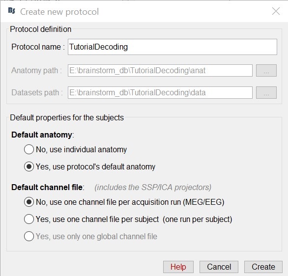
Select the menu File > Create new protocol. Name it "TutorialDecoding" and select the options:
"Yes, use protocol's default anatomy",
"No, use one channel file per condition".
Import the recordings
- Go to the "functional data" view (sorted by subjects).
Right-click on the TutorialDecoding folder > New subject > Subject01
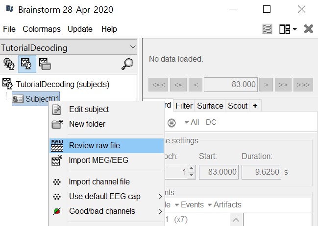
Leave the default options you defined for the protocol.Right click on the subject node (Subject01) > Review raw file.
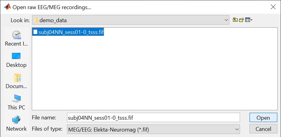
Select the file format: "MEG/EEG: Neuromag FIFF (*.fif)"
Select the file: subj04NN-sess01-0_tsss.fif
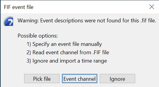
Select "Event channels" to read the triggers from the stimulus channel.
- We will not pay attention to MEG/MRI registration because we are not going to compute any source models. The decoding is done on the sensor data.
Double click on the 'Link to raw file' to visualize the raw recordings. Event codes 13-24 indicate responses to face images, and we will combine them to a single group called 'faces'. To do so, select events 13-24 and from the menu select "Events > Duplicate groups". Then select "Events > Merge groups". The event codes are duplicated first so we do not lose the original 13-24 event codes.
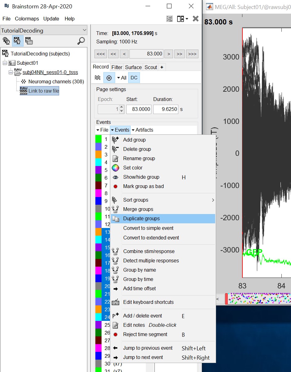
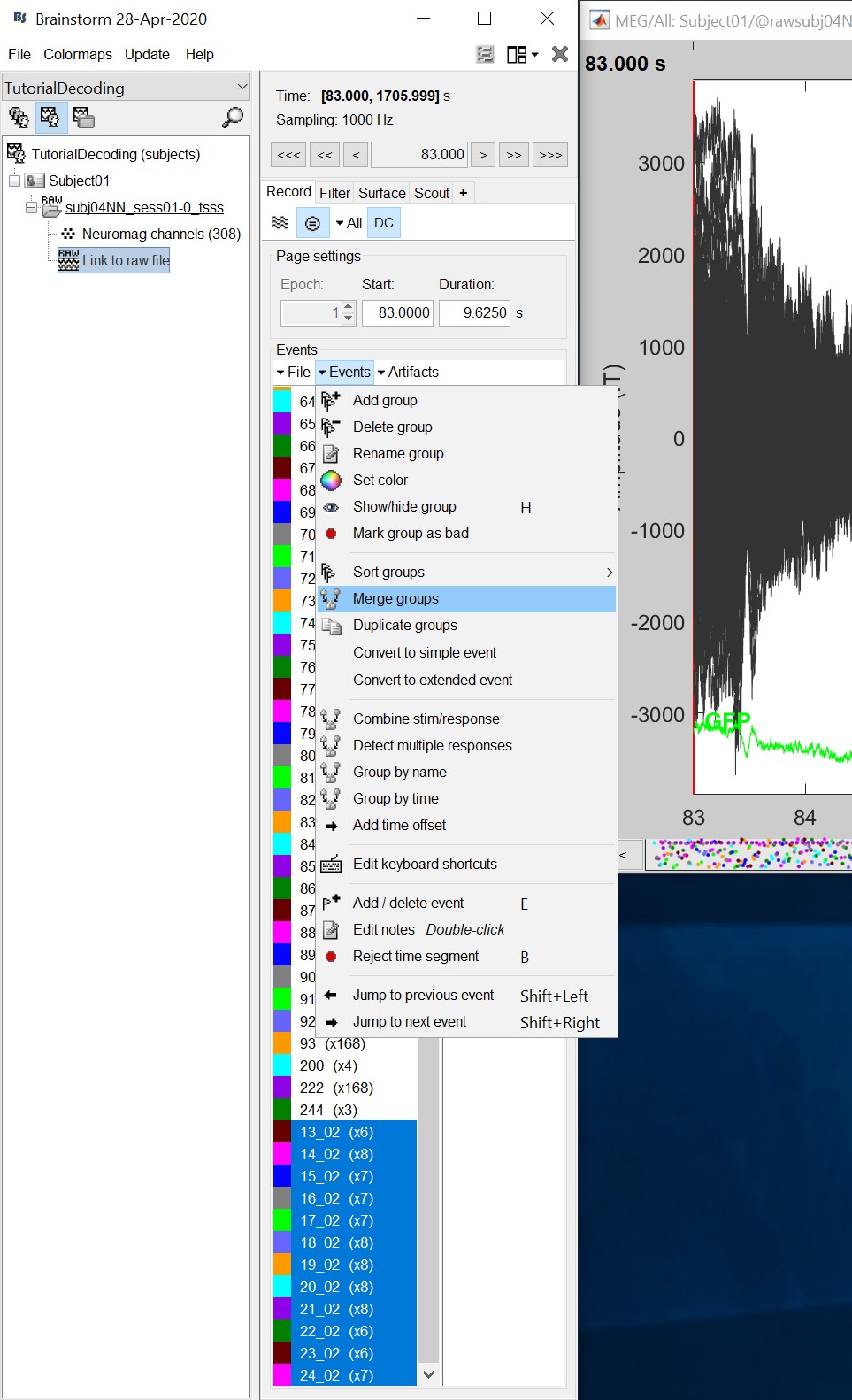
Event codes 49-60 indicate responses to object images, and we will combine them to a single group called 'objects'. To do so, select events 49-60 and from the menu select Events->Duplicate groups. Then select Events->Merge groups. No screenshots are shown since this is similar to above.
We will now import the 'faces' and 'objects' responses to the database. Select "File > Import in database".
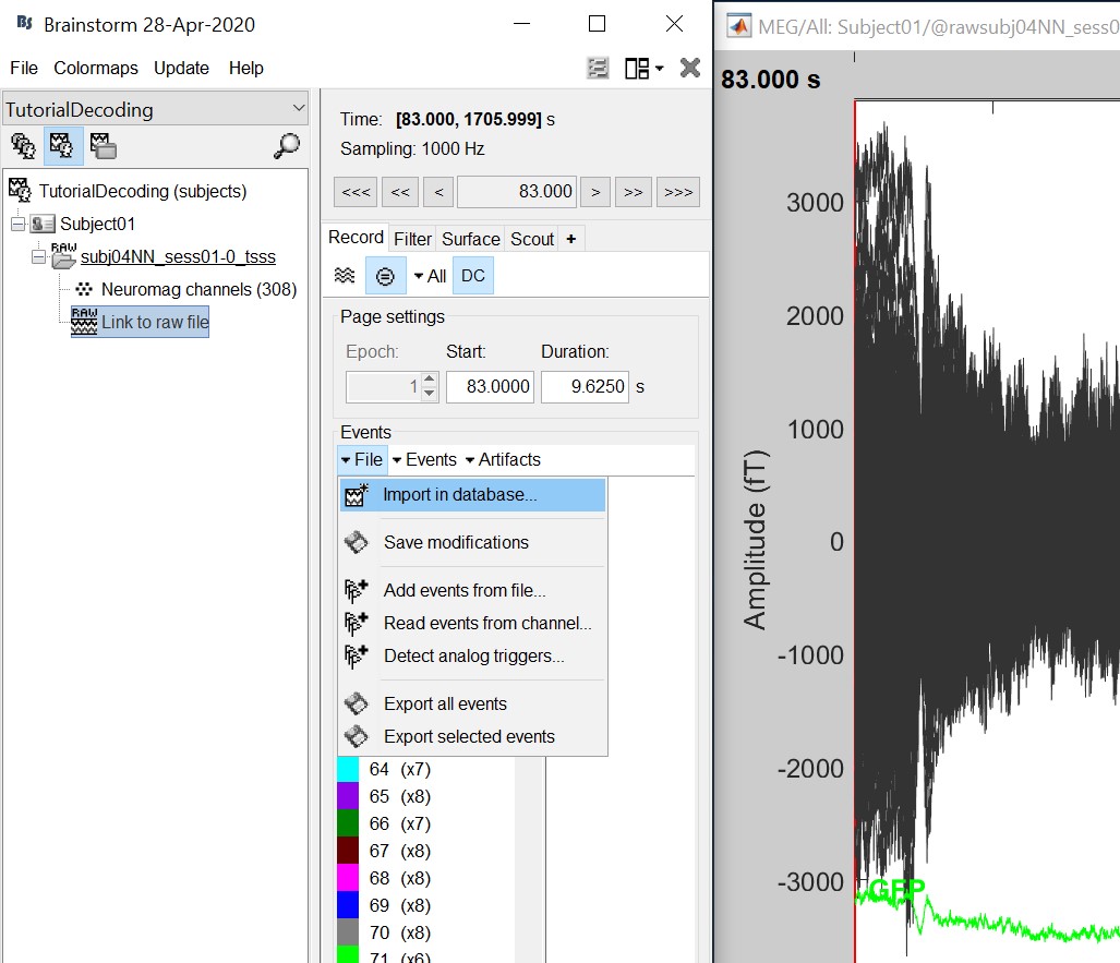
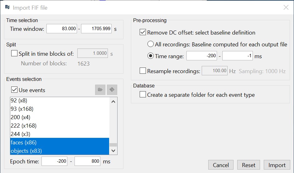
- Select only two events: 'faces' and 'objects'
- Epoch time: [-200, 800] ms
- Remove DC offset: Time range: [-200, 0] ms
Do not create separate folders for each event type
Select files
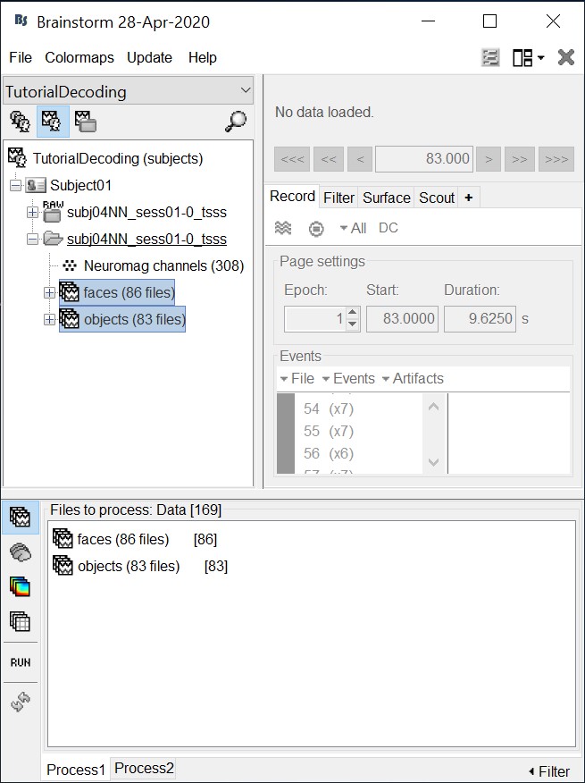
- Drag and drop all the face and object trials to the Process1 tab at the bottom of the Brainstorm window.
Intuitively, you might have expected to use the Process2 tab to decode faces vs. objects. But the decoding process is designed to also handle pairwise decoding of multiple classes (not just two classes) for computational efficiency, so more that two categories can be entered in the Process1 tab.
Decoding with cross-validation
Cross-validation is a model validation technique for assessing how the results of our decoding analysis will generalize to an independent data set.
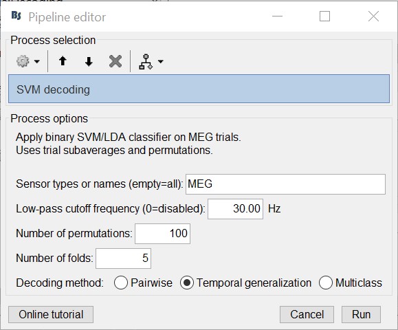
Select process "Decoding > SVM decoding"
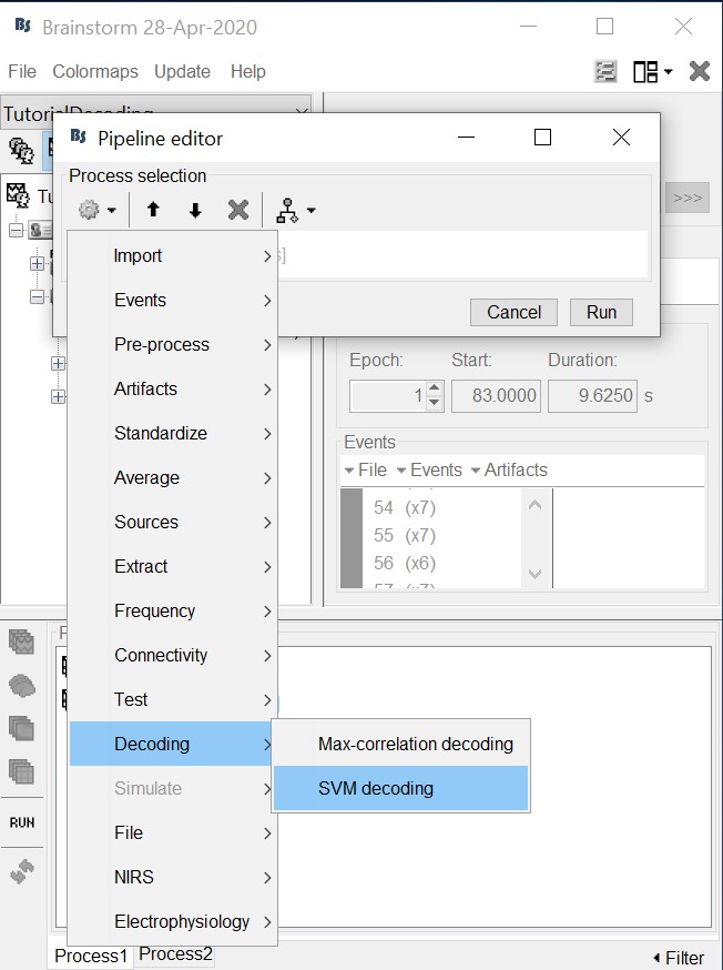
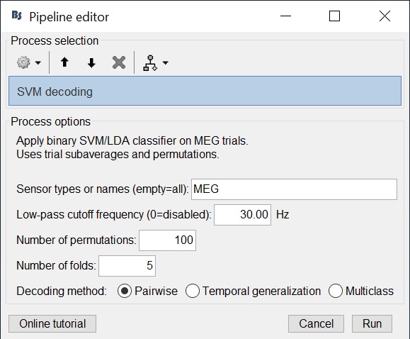
- Select 'MEG' for sensor types
- Set 30 Hz for low-pass cutoff frequency. Equivalently, one could have applied a low-pass filters to the recordings and then run the decoding process. But this is a shortcut to apply a low-pass filter just for decoding without permanently altering the input recordings.
SVM decoding requires the LibSVM toolbox (download and add to your path).
- Select 100 for number of permutations. Alternatively use a smaller number for faster results.
- Select 5 for number of k-folds
- Select 'Pairwise' for decoding. Hint: if more that two classes were input to the Process1 tab, the decoding process will perform decoding separately for each possible pair of classes. It will return them in the same form as Matlab's 'squareform' function (i.e. lower triangular elements in columnwise order)
- The decoding process follows a similar procedure as Pantazis et al. (2018). Namely, to reduce computational load and improve signal-to-noise ratio, we first randomly assign all trials (from each class) into k folds, and then subaverage all trials within each fold into a single trial, thus yielding a total of k subaveraged trials per class. Decoding then follows with a leave-one-out cross-validation procedure on the subavaraged trials.
For example, if we have two classes with 100 trials each, selecting 5 number of folds will randomly assign the 100 trials in 5 folds with 20 trials each. The process than will subaverage the 20 trials yielding 5 subaveraged trials for each class.
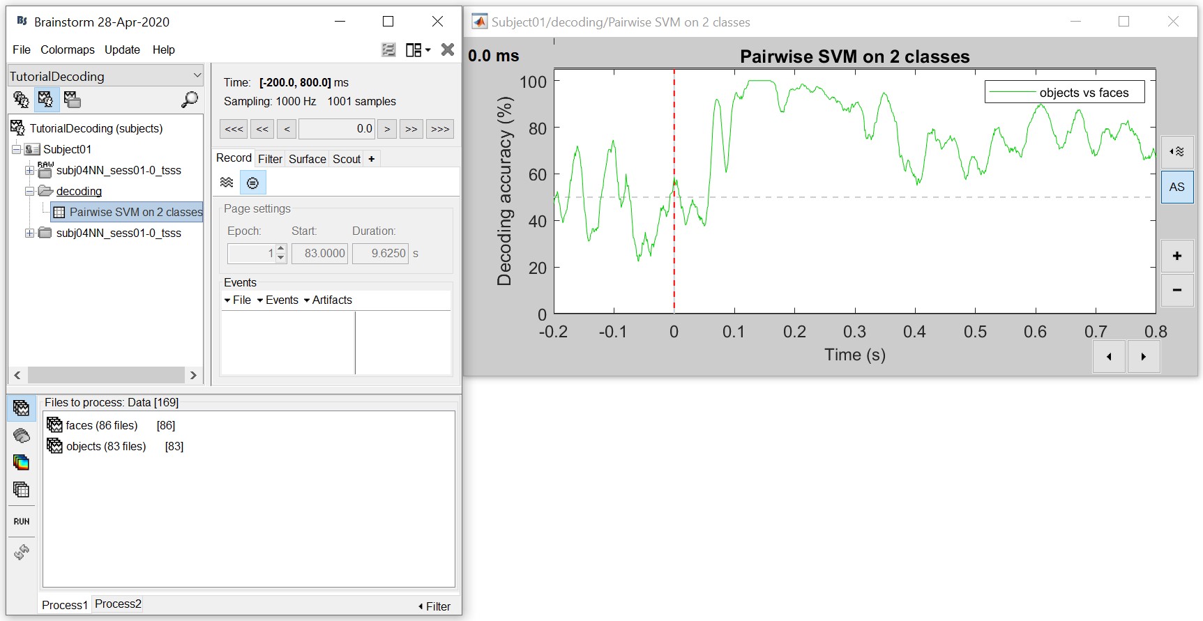
- The process will take some time. The results are then saved in a file in the 'decoding' folder
- For temporal generalization, repeat the above process but select 'Temporal Generalization'.
folder.
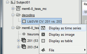
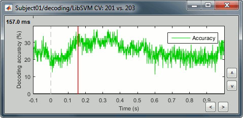
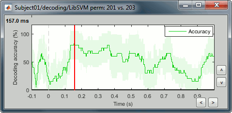
If you double click on it you will see a decoding curve across time.
Permutation
This is an iterative procedure. The training and test data for the SVM/LDA classifier are selected in each iteration by randomly permuting the samples and grouping them into bins of size n (you can select the trial bin sizes). In each iteration two samples (one from each condition) are left out for test. The rest of the data are used to train the classifier with.
Select process "Decoding > Classification with cross-validation". Set options as below:
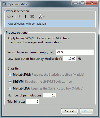
Trial bin size: If greater than 1, the training data will be randomly grouped into bins of the size you determine here. The samples within each bin are then averaged (we refer to this as sub-averaging); the classifier is then trained using the averaged samples. For example, if you have 40 faces and 40 scenes, and you set the trial bin size to 5; then for each condition you will have 8 bins each containing 5 samples. Seven bins from each condition will be used for training, and the two left-out bins (one face bin, one scene bin) will be used for testing the classifier performance.
The results are saved in a file in the new decoding folder.
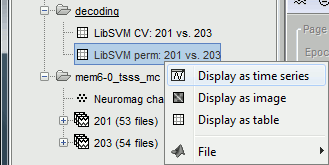
Right-click > Display as time series (or double click).
Acknowledgment
This work was supported by the McGovern Institute Neurotechnology Program to PIs: Aude Oliva and Dimitrios Pantazis. http://mcgovern.mit.edu/technology/neurotechnology-program
References
Khaligh-Razavi SM, Bainbridge W, Pantazis D, Oliva A (2016)
From what we perceive to what we remember: Characterizing representational dynamics of visual memorability. bioRxiv, 049700.Cichy RM, Pantazis D, Oliva A (2014)
Resolving human object recognition in space and time, Nature Neuroscience, 17:455–462.
Additional documentation
Forum: Decoding in source space: http://neuroimage.usc.edu/forums/showthread.php?2719
